
Game-Theoretic Applications of Pentagonal Fuzzy Numbers through New Representation and Defuzzification Schemes
Abstract
in the uncertainty theory. [11, 12] analyzed numerous procedures. Type 2 fuzzy sets
or interval-valued fuzzy sets designed by [29]. [3, 4] submitted intuitionistic fuzzy sets.
[27] evolved fuzzy multi-sets. [24] delivered the concept of neutrosophic fuzzy sets.
[5] specified the probability distribution of the objective function in light of parame-
ters expressed as fuzzy triangular numbers. [8] suggested a new technique for ranking
fuzzy numbers based on length. [14] supplied the theoretical basis of fuzzy numbers,
which was associated with the possibility and Dempster-Shafer theories and conveyed
various types of fuzzy number expressions. [9] suggested a novel arithmetic notion
and process for conducting arithmetic operations on triangular-fuzzy numbers. [16] depicted fuzzy arithmetic operations to eradicate some of the ambushes of the classical
approach. From the perspective of analytical geometry, [25] designated the centroid
formulae for fuzzy numbers. [2] offered a defuzzification using the two fuzzy number’s
distance minimizer. Several modes of ordering trapezoidal fuzzy numbers were con-
ceived by [1]. [19] submitted trapezoidal intuitionistic fuzzy numbers (IF numbers)
and revealed some of its operations. Some further arithmetic operators of the trape-
zoidal fuzzy numbers utilized in [26] suggested an efficient explanation for fuzzy risk
investigation. [7] furnished a novel hazard analysis procedure based on a new tool for
generalized hierarchies. A novel resolution to a typical fuzzy transportation problem
was originated by [15]. [21] analyzed symmetric fuzzy numbers, specified an equivalent
definition of convex fuzzy sets, and proposed a technique for creating a symmetric con-
vex fuzzy set. [17] proclaimed that no underlying membership functions were needed
and explained many aggregation operators. A further procedure for defuzzifying gen-
eralized fuzzy numbers was designed by [22]. [18] presented and approximated many
strategies for total ordering in the intuitionistic fuzzy numbers (IFNs) category. [10]
suggested ranking fuzzy numbers with widely deviating stretches. [13] presented an
alternate technique for estimating additional arithmetic operations of a system using
the sigmoidal number under the fuzzy background. [23] involved fuzzy arithmetic oper-
ations to equations employed to describe anticipation in multiple applications. The
idea of pentagonal-fuzzy number (PFN) was submitted in a broad insight by [20].[6]
formulated pentagonal-fuzzy numbers with other expressions to analyze the conse-
quence of optimal strategies for the candidates in real game situations.
This article covers all defuzzification formulas, expressions, and techniques by consid-
ering the continuity of membership functions. The solution to the game problem is
ultimately detected, and the results are compared to [6]. Subsequently, the present This article is prepared: Section 2 includes preliminaries and pentagonal-fuzzy num-paper provides the updated version of optimal strategies and values of matrix games bers with various expressions, and their α cuts are consulted in Section 3. Section mentioned in [6].
4 contracts with three defuzzification procedures of linear pentagonal fuzzy numbers
with symmetry. In Section 5 hierarchy of pentagonal-fuzzy numbers is depicted. Three
numerical illustrations and suggested defuzzification approaches have numerically
resembled in Section 6. Section 7 finishes with the conclusion of this paper.
2. Preliminaries
In this section, we recall some basic definitions and notations which are useful
throughout the paper.
Definition 1. A fuzzy set A ˜ is the collection of ordered pairs (x, µ (x)) defined on
the universal set X and denoted by A ˜ = {(x, µ (x))|x ∈ X and µ (x) ∈ [0, 1]}, where
A ˜ A ˜
µ : X → [0, 1] is the membership function of A ˜It is commonly believed that all
details accessed by the entities are represented in crisp numbers. However, most real-
life systems are engaged when the goals and constraints are often vague or unclear.
Definition 2. An interval valued fuzzy set A ˜ defined on the universal set X is
represented by A ˜ = {(x, (µ (x), µ (x))) |x ∈ X}, where µ : X → [0, λ] and
A ˜U A ˜L A ˜U µ ˜L : X → [0, ω] are the upper and lower membership functions with the maximum
values λ and ω respectively.
Definition 3. A non linear interval valued triangular fuzzy number A ˜ is
nLIV F N
denoted by A ˜ = [{(a , b, c ; λ) , (a, b, c; ω)}; ξ , ξ , ξ , ξ ] where 0 < ω ≤ λ ≤ 1
nLIV F N 1 1 1 2 3 4
and a1 < a < b < c < c1. The upper and lower membership functions are defined as
follows: ξ
x−a1 λ ; a1 ≤ x ≤ b b−a1 λ ; x = b µ ˜U (x) = (1)
A ξ2
c1−x λ ; b ≤ x ≤ c c −b 1 0 ; else
and x−a ω ; a ≤ x ≤ b b−a ω ; x = b µ ˜L (x) = (2)
A ξ4
c−x ω ; b ≤ x ≤ c c−b 0 ; else
3. Pentagonal fuzzy number and its different
representations
Within this section, we have established distinct categories of pentagonal fuzzy num-
bers by leveraging the continuity of the membership function—a dimension that was
notably absent in the framework presented by [6].
Definition 4. A pentagonal fuzzy number with µ ˜(x) as membership function is
represented by A ˜ = (a , a , a , a , a ) and satisfies the following conditions:
1 2 3 4 5
1. µ ˜(x) is continuous in [0, 1].
2. µ ˜(x) is strictly increasing continuous function on [a1, a2] and [a2, a3].
3. µ ˜(x) is strictly decreasing continuous function on [a3, a4] and [a4, a5].
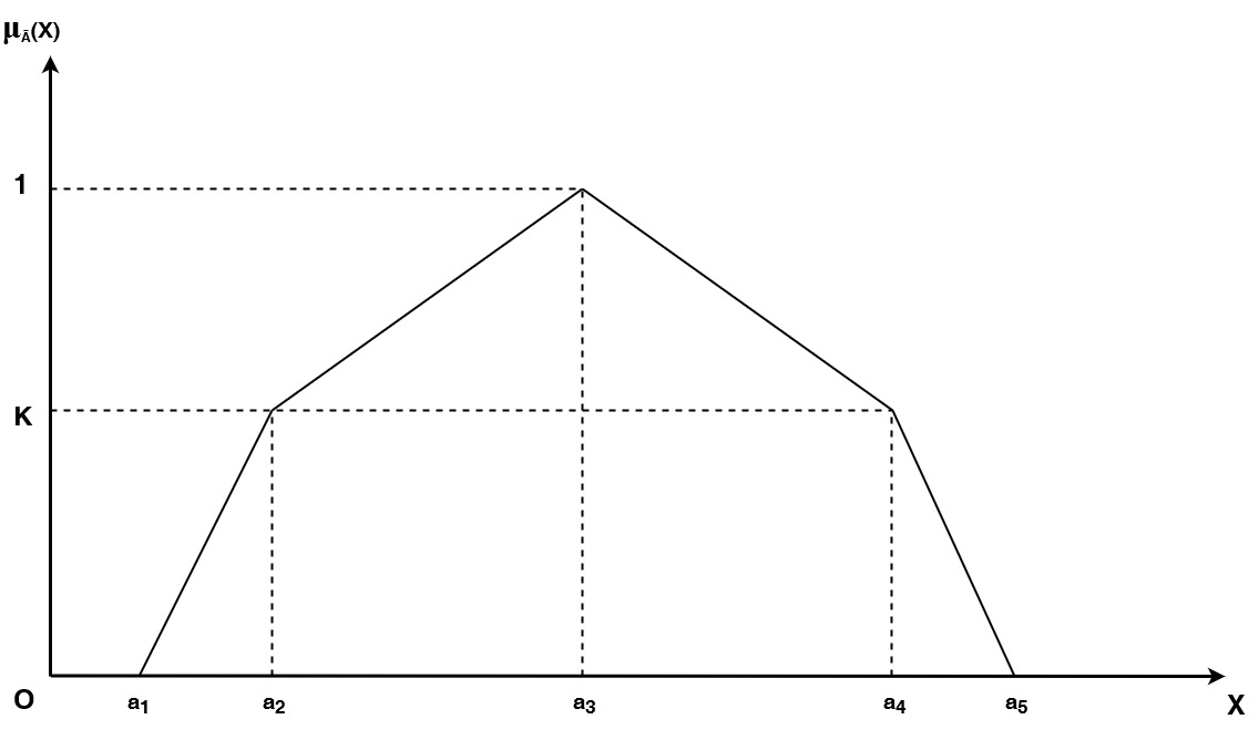
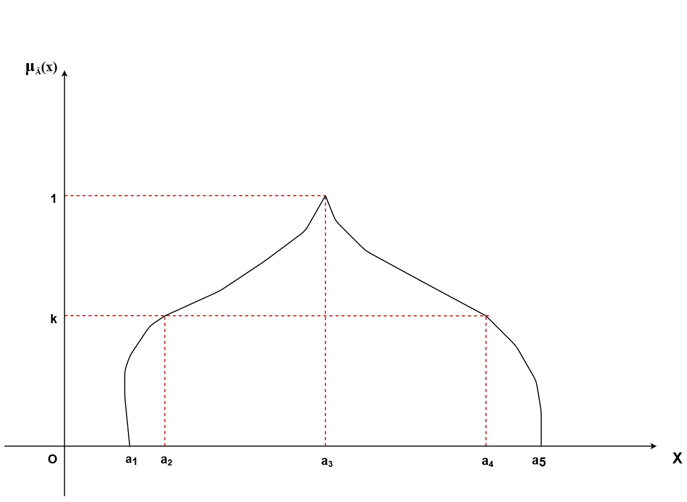
Definition 5. Linear pentagonal fuzzy number with symmetry (LS) is represented by
A ˜ = ⟨a , a , a , a , a ; k⟩. The revised definition by the Figure 1 with a continuous
LS 1 2 3 4 5
membership function is given as follows:
x−a1 k ; a1 ≤ x ≤ a2 a2−a1 x−a k + (1 − k) ; a2 ≤ x ≤ a3 a3−a2 1 ; x = a3 µ ˜ (x) = (3)
ALS a −x
k + (1 − k) ; a3 ≤ x ≤ a4 a4−a3 a −x k ; a4 ≤ x ≤ a5 a5−a4 0 ; else Fig. 1 Linear PFN with symmetry (LS).
Definition 6. The revised α-cut of linear pentagonal fuzzy number with symmetry is defined as the collection of all x ∈ X having membership function µ ˜ (x) as greater
A LS
than or equal to α i.e. Aα = {x ∈ X|µ ˜ (x) ≥ α} is given by
ALS
A1L(α) = a1 + (a2 − a1) ; α ∈ [0, k] α−k A2L(α) = a2 + (a3 − a2) ; α ∈ [k, 1] Aα = α−k (4) A2R(α) = a4 − (a4 − a3) ; α ∈ [k, 1] 1−k A1R(α) = a5 − (a5 − a4) ; α ∈ [0, k]
Here A1L(α), A2L(α) are the increasing functions of α and A1R(α), A2R(α) are the
decreasing functions of α.
Definition 7. Non linear pentagonal fuzzy number with symmetry (N S) is represented
by A ˜ = (a , a , a , a , a ; k) . The revised definition by the Figure 2 with
N S 1 2 3 4 5 (ξ ,ξ ;ζ ,ζ )
1 2 1 2
a continuous membership function is given as follows:
x−a1 k ; a1 ≤ x ≤ a2 a2−a1 ξ2 x−a k + (1 − k) ; a2 ≤ x ≤ a3 a3−a2 1 ; x = a3 µ ˜ (x) = ζ (5)
AN S 1
a4−x k + (1 − k) ; a ≤ x ≤ a a −a 3 4 ζ2 a5−x k ; a4 ≤ x ≤ a5 a −a 5 4 0 ; else Fig. 2 Non Linear PFN with Symmetry A ˜
NS.
Definition 8. The revised α-cut of non linear pentagonal fuzzy number with symmetry
is defined as the collection of all x ∈ X with membership function µ ˜ (x) as greater
AN S
than or equal to α i.e. Aα = {x ∈ X|µ ˜ (x) ≥ α} is
AN S
α k (a2 − a1) ; α ∈ [0, k] A1L(α) = a1 + 1
α−k (a − a ) ; α ∈ [k, 1] A2L(α) = a2 + 1−k 3 2 (6) Aα = α−k A (α) = a − 1−k (a4 − a3) ; α ∈ [k, 1] 2R 4 α 2 A (α) = a − k (a5 − a4) ; α ∈ [0, k] 1R 5
Here A1L(α), A2L(α) are the increasing functions of α and A1R(α), A2R(α) are the
decreasing functions of α.
Definition 9. The revised definition of linear interval valued pentagonal fuzzy num-
ber with symmetry (LIP S) A ˜ = ⟨(a , a , c, a , a ; k, p) , (b , b , c, b , b ; w, q)⟩ is
LIP S 1 2 4 5 1 2 4 5 defined by the Figure 3 with upper and lower membership functions as follows:
x−a1 p ; a1 ≤ x ≤ a2 a2−a1 x−a p + (k − p) ; a2 ≤ x ≤ c c−a2 k ; x = c µ ˜U (x) = (7)
A a −x
LIP S 4 p + (k − p) ; c ≤ x ≤ a4 a4−c a −x p ; a4 ≤ x ≤ a5 a5−a4 0 ; else
and x−b1 q ; b1 ≤ x ≤ b2 b2−b1 x−b q + (w − q) ; b2 ≤ x ≤ c c−b2 w ; x = c µ ˜L (x) = (8)
A b −x
LIP S 4 q + (w − q) ; c ≤ x ≤ b4 b4−c b −x q ; b4 ≤ x ≤ b5 b5−b4 0 ; else
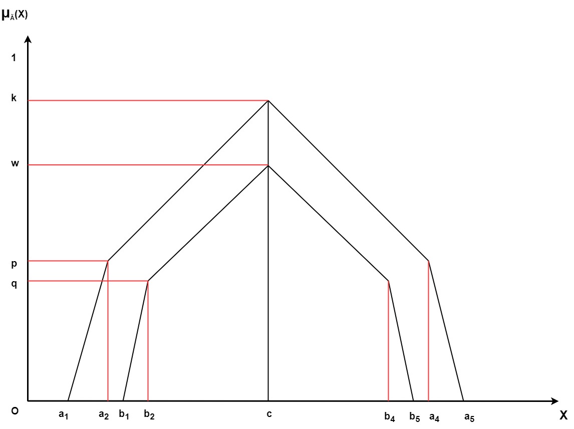
Definition 10. The revised α-cut of linear interval valued pentagonal fuzzy number
˜ ˜U ˜L with symmetry is defined as ALIP Sα = ALIP S ⊖ ALIP S for α1 ∈ [0, w];
α α2 α α1 α2 ∈ [0, k].
Where U α2 (a − a ) ; α ∈ [0, p] A (α ) = a + p 2 1 2 1L 2 1 U α2−p A (α ) = a + (c − a2) ; α2 ∈ [p, k] 2L 2 2 k−p (9) ˜U U α2−p A = A (α ) = a − (a4 − c) ; α2 ∈ [p, k]
LIP S 2R 2 4 k−p
α2 α U 2 (a − a ) ; α ∈ [0, p] A 1R(α2) = a5 − p 5 4 2
and L α1 (b − b ) ; α ∈ [0, q] A (α ) = b + q 2 1 1 1L 1 1 L α1−q A (α ) = b + (c − b2) ; α1 ∈ [q, w] 2L 1 2 w−q (10) ˜L L α1−q A = A (α ) = b − (b4 − c) ; α1 ∈ [q, w]
LIP S 2R 1 4 w−q
α1 α L 1 (b − b ) ; α ∈ [0, q] A 1R(α1) = b5 − q 5 4 1
U U L L
Here A 1L(α2), A 2L(α2), A 1L(α1), A 2L(α1) are the increasing functions of
U U L L
α2 and α1 correspondingly and A 1R(α2), A 2R(α2), A 1R(α1), A 2R(α1) are the
decreasing functions of α2 and α1 correspondingly.
Definition 11. The membership functions of linear interval val-
ued pentagonal fuzzy number with asymmetry (LIP AS) A ˜ =
LIP AS
⟨(a1, a2, c, a4, a5; k, p, r) , (b1, b2, c, b4, b5; w, q, s)⟩ are defined by the Figure 4 with upper
and lower membership functions as follows:
; a1 ≤ x ≤ a2 a2−a1 x−a1 p x−a2 ; a ≤ x ≤ c p + (k − p) c−a 2
k ; x = c (11)
a4−x ; c ≤ x ≤ a4 r + (k − r) a4−c µ ˜U (x) = a −x A 5 ; a ≤ x ≤ a LIP AS r a −a 4 5 5 4
0 ; else
and x−b ; b1 ≤ x ≤ b2 b2−b1 1 x−b2 q + (w − q) ; b2 ≤ x ≤ c c−b2 w ; x = c (12)
b4−x ; c ≤ x ≤ b4 µ ˜L (x) = s + (w − s) b4−c LIP AS b5−x ; b ≤ x ≤ b s b −b 4 5 5 4 0 ; else
Definition 12. The revised α-cut of linear interval valued pentagonal fuzzy number
˜U ˜L with asymmetry is defined as ALIP ASα = ALIP AS ⊖ ALIP AS for α1 ∈
α α2 α α1
[0, w]; α2 ∈ [0, k].
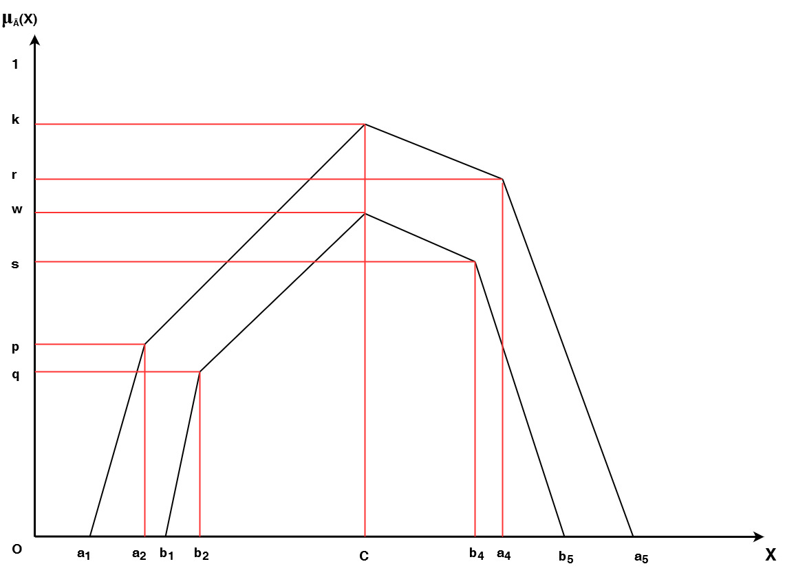
Where
U α2
A (α ) = a + (a2 − a1) ; α2 ∈ [0, p] 1L 2 1 p α −p U 2 A (α ) = a + (c − a2) ; α2 ∈ [p, k] U 2L 2 2 k−p (13) A ˜ = U α −r LIP AS 2 (a − c) ; α ∈ [r, k] A 2R(α2) = a4 − k−r 4 2 α2 U α 2 (a − a ) ; α ∈ [0, r] A 1R(α2) = a5 − r 5 4 2
and L α1 (b − b ) ; α ∈ [0, q] A (α ) = b + q 2 1 1 1L 1 1 L α1−q A (α ) = b + (c − b2) ; α1 ∈ [q, w] 2L 1 2 w−q (14) ˜L α −s A = L 1 (b − c) ; α ∈ [s, w] LIP AS A 2R(α1) = b4 − w−s 4 1 α1 L α1 A (α ) = b − (b5 − b4) ; α1 ∈ [0, s]
1R 1 5 s U U L L
Here A 1L(α2), A 2L(α2), A 1L(α1), A 2L(α1) are the increasing functions of
U U L L
α2 and α1 correspondingly and A 1R(α2), A 2R(α2), A 1R(α1), A 2R(α1) are the
decreasing functions of α2 and α1 correspondingly.
Definition 13. The membership functions of non linear interval val-
ued pentagonal fuzzy number with symmetry (N IP S) A ˜ = D E N IP S
(a1, a2, c, a4, a5; k, p) , (b1, b2, c, b4, b5; w, q) are defined by the Figures 5 to 8 for different (ξ1,ξ2;ζparameters 1,ζ2) ξ1, ξ2, ζ1, ζ2 with (ξ1,ξrevised 2;ζ1,ζ2) continuous upper and
lower membership functions as follows:
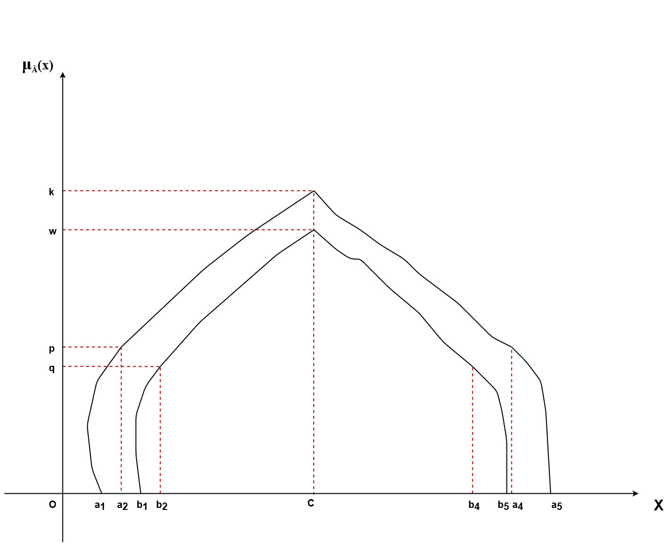
NIPS 1 2 1 2
x−a1 ξ1 ; a1 ≤ x ≤ a2 a2−a1
x−a2 ; a ≤ x ≤ c p + (k − p) c−a 2 k ; x = c (15) µ ˜U (x) = ζ1 N IP S a4−x ; c ≤ x ≤ a4 p + (k − p) a4−c
a5−x ; a ≤ x ≤ a p a −a 4 5
0 ; else
and ξ1 ; b1 ≤ x ≤ b2 bx 2− −bb1 1 q ξ x−b2 ; b ≤ x ≤ c q + (w − q) c−b 2 w ; x = c (16) ζ1 b4−x ; c ≤ x ≤ b4 µ ˜L (x) = q + (w − q) b4−c N IP S 2 b5−x ; b ≤ x ≤ b q b −b 4 5 5 4 0 ; else
Definition 14. The revised α-cut of non linear interval valued pentagonal fuzzy num-
˜U ˜L ber with symmetry is defined as follow: AN IP Sα = AN IP S ⊖ AN IP S for
α α2 α α1
α1 ∈ [0, w]; α2 ∈ [0, k].
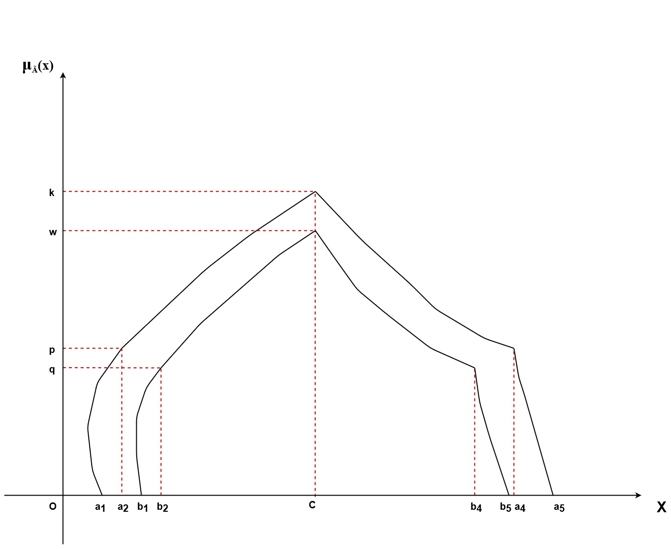
NIPS 1 2 1 2
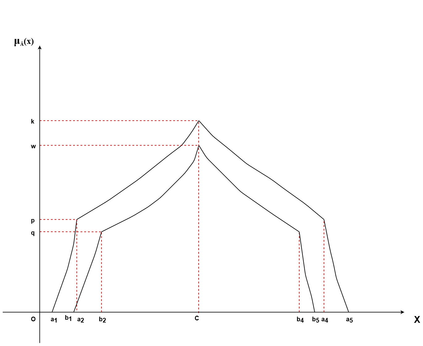
NIPS 1 2 1 2 NIPS 1 2 1 2
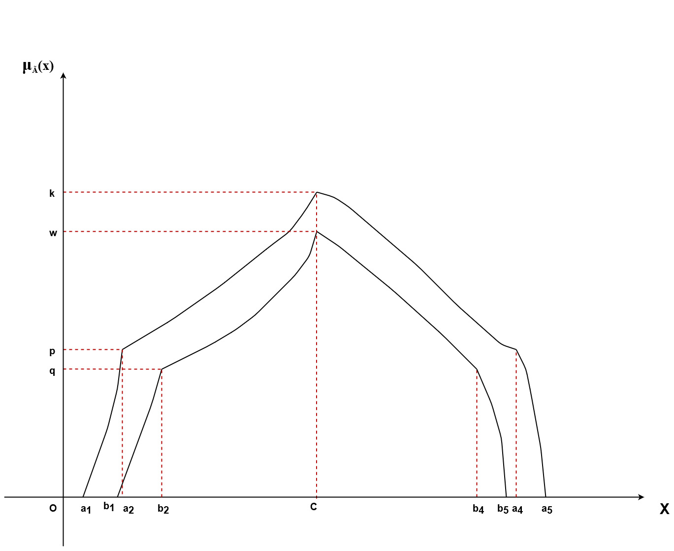
Where
U α2 A (α ) = a + p (a2 − a1) ; α2 ∈ [0, p] 1L 2 1 ξ2 U α −p 2 (c − a ) ; α ∈ [p, k] A 2L(α2) = a2 + k−p 2 2 (17) A = ζ1
N IP S U α2−p
α A (α ) = a − k−p (a4 − c) ; α2 ∈ [p, k] 2 2R 2 4
U α2 A (α ) = a − p (a5 − a4) ; α2 ∈ [0, p] 1R 2 5
and 1 L α1 (b2 − b1) ; α1 ∈ [0, q] A (α ) = b + q 1L 1 1 1 α −q L 1 (c − b ) ; α ∈ [q, w] A 2L(α1) = b2 + w−q 2 1 (18) ˜L ζ1 A = L α1−q N IP S A (α ) = b − w−q (b4 − c) ; α1 ∈ [q, w] α1 2R 1 4 ζ2 L α 1 (b − b ) ; α ∈ [0, q] A 1R(α1) = b5 − q 5 4 1
U U L L
Here A 1L(α2), A 2L(α2), A 1L(α1), A 2L(α1) are the increasing functions of
U U L L
α2 and α1 correspondingly and A 1R(α2), A 2R(α2), A 1R(α1), A 2R(α1) are the
decreasing functions of α2 and α1 correspondingly.
Definition 15. The membership functions of non linear interval val-
ued pentagonal fuzzy number with asymmetry (N IP AS) A ˜ =
N IP AS (a1, a2, c, a4, a5; k, p, s) , (b1, b2, c, b4, b5; w, q, t) are defined by
(ξ1,ξ2;ζ1,ζ2) (ξ1,ξ2;ζ1,ζ2)
the Figures 9 to 12 for different parameters ξ1, ξ2, ζ1, ζ2 having continuous upper and
lower membership functions as follows:
x−a1 ξ1 ; a1 ≤ x ≤ a2 a2−a1
x−a2 ; a ≤ x ≤ c p + (k − p) c−a 2 k ; x = c (19) µ ˜U (x) = ζ1 N IP AS a4−x ; c ≤ x ≤ a4 s + (k − s) a4−c
a5−x ; a ≤ x ≤ a s a −a 4 5 5 4 0 ; else
and ξ1 ; b1 ≤ x ≤ b2 bx 2− −bb1 1 q ξ2 x−b2 ; b ≤ x ≤ c q + (w − q) c−b 2 w ; x = c (20)
b4−x ; c ≤ x ≤ b4 µ ˜L (x) = t + (w − t) b4−c N IP AS 2 b −x 5 ; b ≤ x ≤ b t b −b 4 5 5 4 0 ; else
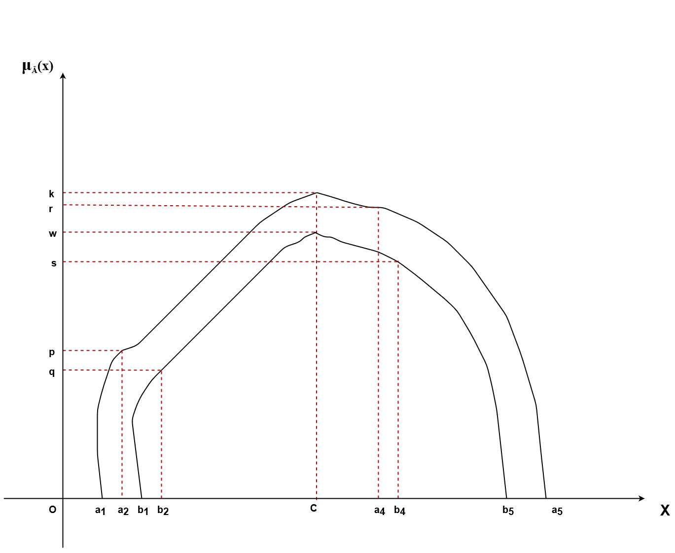
NIPAS 1 2 1 2 NIPAS 1 2 1 2
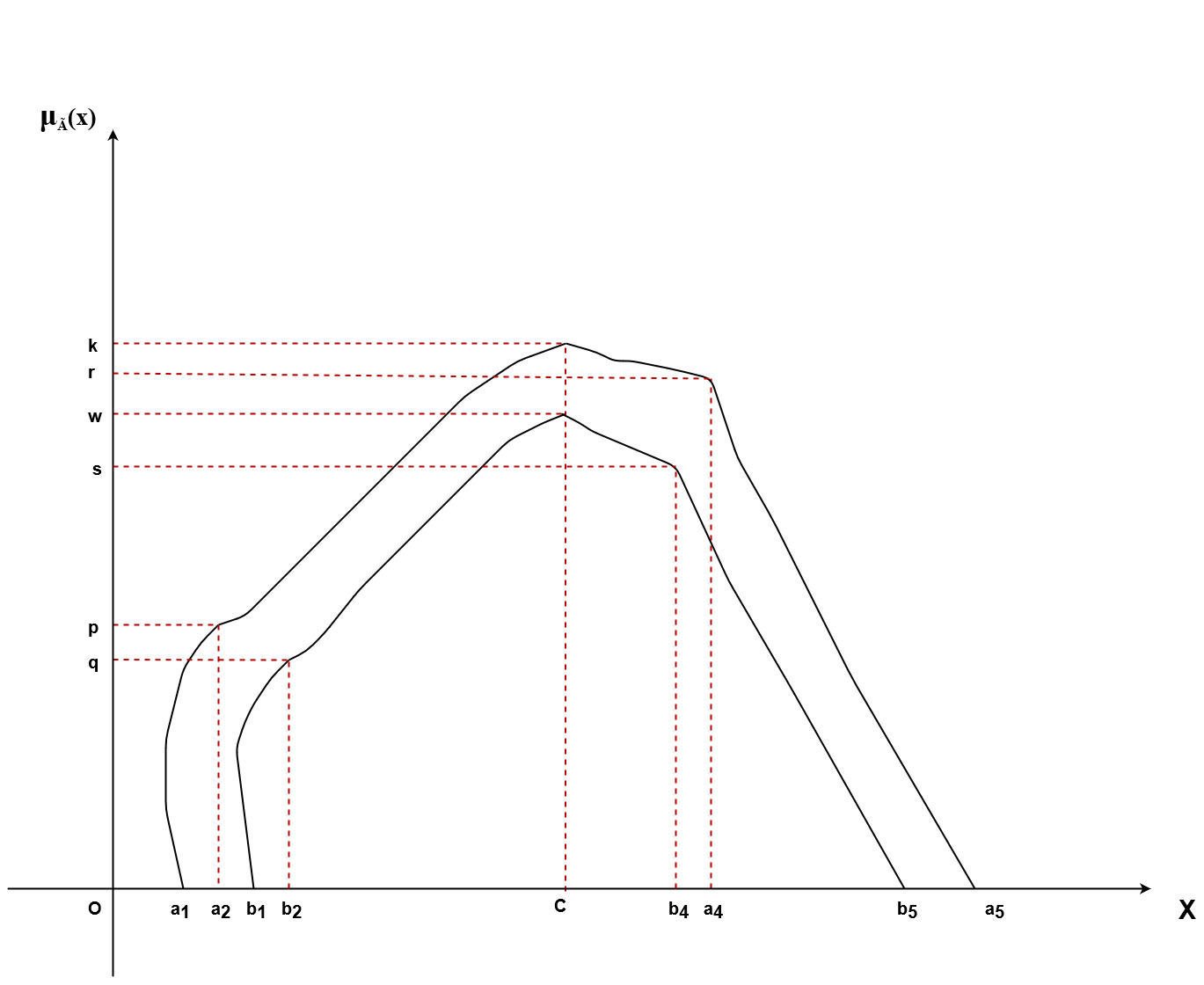
Definition 16. The revised α-cut of non linear interval valued pentagonal fuzzy num-
˜U ˜L ber with asymmetry defined as AN IP ASα = AN IP AS ⊖ AN IP AS for
α α2 α α1
α1 ∈ [0, w]; α2 ∈ [0, k].
Where
α p (a2 − a1) ; α2 ∈ [0, p] U 2 A 1L(α2) = a1 + 1 U α2−p A (α ) = a + k−p (c − a2) ; α2 ∈ [p, k] (21) 2L 2 2 ˜U ζ A = 1 N IP AS U α2−s (a − c) ; α ∈ [s, k] α A (α ) = a − k−s 4 2 2 2R 2 4 U α2 2 A (α ) = a − s (a5 − a4) ; α2 ∈ [0, s] 1R 2 5
and 1
L α1 (b − b ) ; α ∈ [0, q] A (α ) = b + q 2 1 1 1L 1 1 1 ξ2 L α1−q A (α ) = b + w−q (c − b2) ; α1 ∈ [q, w] (22)
2L 1 2
A ˜ =
N IP AS ζ1
α L α1−t (b − c) ; α ∈ [t, w] 1 A (α ) = b − w−t 4 1 2R 1 4 L α1 2 A (α ) = b − t (b5 − b4) ; α1 ∈ [0, t] 1R 1 5 NIPAS 1 2 1 2
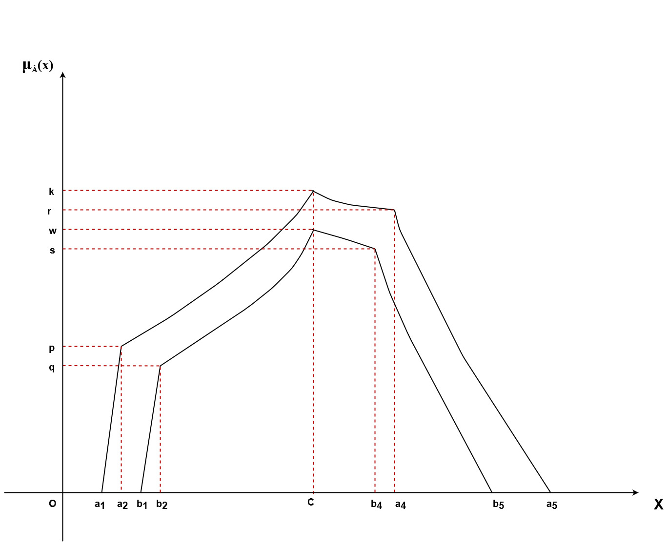
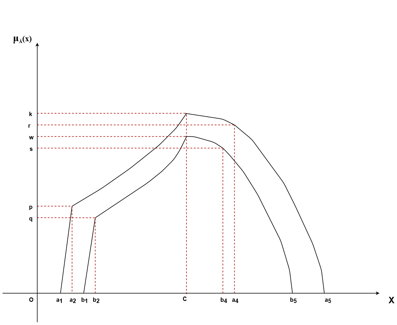
NIPAS 1 2 1 2 U U L L
Here A 1L(α2), A 2L(α2), A 1L(α1), A 2L(α1)”are the increasing functions of
U U L L
α2 and α1 correspondingly and A 1R(α2), A 2R(α2), A 1R(α1), A 2R(α1) are the
decreasing functions of α2 and α1 correspondingly.
4. Defuzzification
The defuzzification method converts the fuzzy inference result into an appropriate
exact value. It plays a critical role in a fuzzy environment. For fuzzy logic, several
defuzzification techniques are available, such as the center of the area (centroid), great-
est of maxima, smallest of maxima, mean of maxima, the bisector of area, graded
mean integral value, and so on. We investigate three methods to defuzzify the linear
pentagonal fuzzy number with symmetry (LS) based on different approaches. Our
results are compared with [6].
4.1 Centroid Method
In this section we have proposed R a methodR for the defuzzification R of non linear
a2 a3 a4 a5
xµ ˜ (x)dx+ xµ ˜ (x)dx+ xµ ˜ (x)dx+ xµ ˜ (x)dx a1 R AN S a R2 AN S Ra3 AN S R a4 AN S
a2 a3 a4 a5
pentagonal fuzzy number µ (with x)dx+symmetry µ (x) as dx+ follows: µ (x)dx+ µ (x)dx (23)
a A ˜ a A ˜ a A ˜ a A ˜ 1 N S 2 N S 3 N S 4 N S
= R Q
From Eqs. (5) and (23) we obtain " # Z " # Z ξ1 a ξ2
a2 3
x − a1 x − a2 P = x k dx + x k + (1 − k) dx a2 − a1 a a3 − a2
a1 2
# Z " # " ζ1 a ζ2 a4 a5 − x a4 − x dx + x k dx + x k + (1 − k) a − a a − a
4 3 a4 5 4
# Z " # and " ξ1 a3 ξ2 Z a x − a2 x − a1 dx + k + (1 − k) dx Q = k a2 − a1 a a3 − a2 # Z " # a1 " ζ ζ
1 a5 2
Z a a − x a4 − x dx + k dx + k + (1 − k) a − a a − a
4 3 a4 5 4
On computing we have
2 2 2
k(a −a ) k(a3 −a2 ) (1−k)a (a −a )
2 1 3 3 2
ka (a −a ) − + +
2 (ξ1+1) 2 1 (ξ1+1)(ξ1+2) 2 (ξ2+1)
P = 2 2 2 k(a4 −a3 ) (1−k)a (a −a ) (24)
(1−k)(a −a ) 3 4 3
3 2 + + − (ξ2+1)(ξ2+2) 2 (ζ1+1)
2 ka4(a5−a4) k(a5−a4) (1−k)(a4−a3)
+ + +
(ζ1+1)(ζ1+2) (ζ2+1) (ζ2+1)(ζ2+2) and
(1−k)(a3−a2) (1−k)(a4−a3)
k(a2−a1) + k (a − a ) + + k (a − a ) + Q = (ξ +1) 3 2 (ξ +1) 4 3 (ζ +1) 1 2 1 (25)
k(a5−a4)
+ (ζ +1)
If we set ξ1 = 1, ξ2 = 1, ζ1 = 1 and ζ2 = 1 then the proposed defuzzification technique
applies for the linear pentagonal fuzzy number with symmetry as follows
(26) L + NM
where
2 2 2 2
k(a −a ) k(a3 −a2 ) (1−k)a (a −a ) (1−k)(a −a ) 2 1 3 3 2 3 2 (27) − + + −
ka2(a2 2−a1) 6 2 2 6
2 2 (1−k)a3(a4−a3) (1−k)(a4−a3) ka4(a5−a4) k(a5−a4)
k(a4 −a3 ) (28) + + + + M = 2 2 6 2 6 and (1−k)(a −a ) k(a2−a1) + k (a − a ) + + k (a − a ) N = 2 3 2 2 4 3 (29)
k(a5−a4) (1−k)(a4−a3)
For k = 1 we have
2 2 2 2 (30) a4 + a5 + a4a5 − a1 − a2 − a1a2 R = 3 (a4 + a5 − a1 − a2)
4.2 Defuzzification using α-cut
In this section, we propose a method to compute the defuzzification of non-linear
pentagonal D fuzzy numbers with symmetryE as follows:
Since try A ˜ the= left(a and , aright , a , a α-cuts , a ; kof ) a non linear are pentagonal fuzzy number with symme-
N S 1 2 3 4 5 (ξ ,ξ ;ζ ,ζ )
1 2 1 2
−1 α (a − a ); α ∈ [0, k], L (α) = a1 + k
−1 2
R (α) = a5 − (a5 − a4); α ∈ [0, k],
α − k ξ2 L (α) = a2 + (a3 − a2); α ∈ [k,1], 1 − k
α − k ζ1 R (α) = a4 − (a4 − a3); α ∈ [k,1].
1 − k Then the mean of α- cut of A ˜ is
Z 1 −1 −1 L (α) + R (α) dα A ˆ = 2 Z 1 −1 −1 Z kα=0 L (α) + R (α)
−1 −1
L (α) + R (α) dα + dα = 2 2 α=k i α=0 h 1 1
ξ1 α ζ2
Z α (a − a ) + a − (a − a ) k a1 + k 2 1 5 k 5 4 dα
ξ2 ζ1
α−k α−k
Z a + 1−k (a3 − a2) + a4 − 1−k (a4 − a3) dα
α=k k(a5−a4) (1−k)(a3−a2) (1−k)(a4−a3)
k(a2−a1) − + (1 − k) (a + a ) + − k (a + a ) + 2 4
1 5 1 +1 1 +1 1 +1 1 +1
ξ1 ζ2 ξ2 ζ1
(31)
If we set ξ1 = 1, ξ2 = 1, ζ1 = 1 and ζ2 = 1 then the proposed defuzzification technique
applies for the linear pentagonal fuzzy number with symmetry as follows
A ˆ = k(a −a ) (1−k)(a −a ) (1−k)(a −a )
5 4 3 2 4 3
− + (1 − k) (a2 + a4) + −
2 2 2 2 k(a2−a1)
k (a1 + a5) + 2 (32)
For k = 1 we have a1 + a2 + a4 + a5 (33) A ˆ = 4
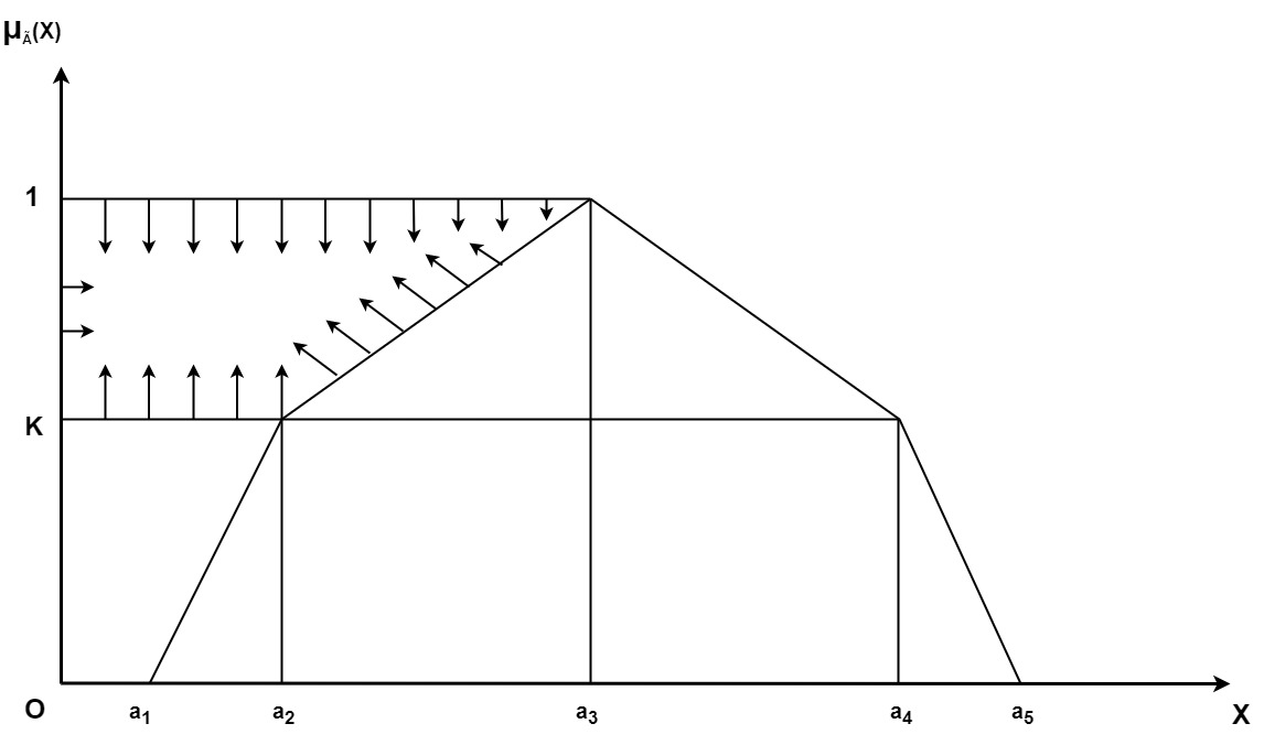
4.3 Defuzzification using Removal of Area Method
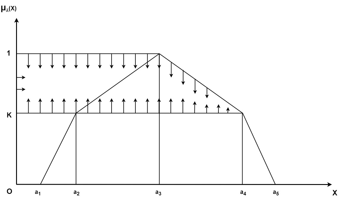
We consider numerous types of regions of the related linear PFN 1 as illustrated below R A, ˆ 0 = Area of the highlighted region for Figure 13 = k (a + a )
1 2 1 2
R2 A, 0 = Area of the highlighted region for Figure 14 = (1 − k) (a2 + a3)
R3 A, 0 = Area of the highlighted region for Figure 15 = (1 − k) (a3 + a4)
R4 A, 0 = Area of the highlighted region for Figure 16 = k (a4 + a5)
Therefore,
R A, ˆ 0 + R A, ˆ 0 + R A, ˆ 0 + R A, ˆ 0
1 2 3 4
R D, ˆ 0 = 4 1 1 1 (34) 1 k (a + a ) + (1 − k) (a + a ) + (1 − k) (a + a ) + k (a + a )
2 1 2 2 2 3 2 3 4 2 4 5
k (a1 + a2) + (1 − k) (a2 + a3) + (1 − k) (a3 + a4) + k (a4 + a5).
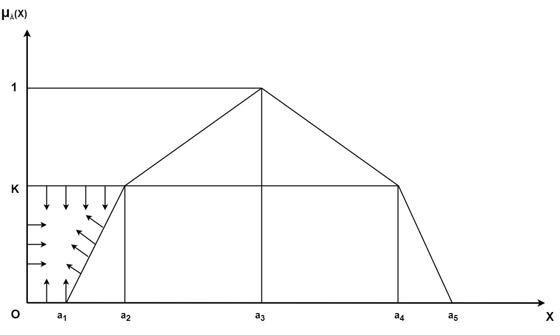
For k = 1, we have a1 + a2 + a4 + a5 R D, ˆ 0 = . (35)
4.4 Comparison of the Above Defuzzification Methods
We compared the above proposed defuzzification methods numerically for suitable
pentagonal fuzzy number.
Table 1. Numerically Comparison of Defuzzification Methods.
This table is shown in the PDF version of the article.
5. Numerical Problems
Example 1. Consider a fuzzy matrix game for two different players A and B whose
pay-offs are linear pentagonal fuzzy numbers with symmetry as follows:
Now using the mean of α- cut method as defuzzification defined by Eq. (32)
for linear pentagonal fuzzy number to convert the given fuzzy pay-off matrix game as Table (1) into the following crisp matrix game as Table 3, we have
The above crisp matrix game defined by Table 3 has no saddle point. Therefore according to the dominance property in matrix games row X1 can be dominated by row X3. Hence we
have a modified matrix game as Table 4.
Again we have that all the elements of column Y1 are greater than or equal to corresponding elements of column Y3. Therefore column Y1 dominates column Y3 and so we can delete the
column Y1 for new improved matrix game as Table 5.
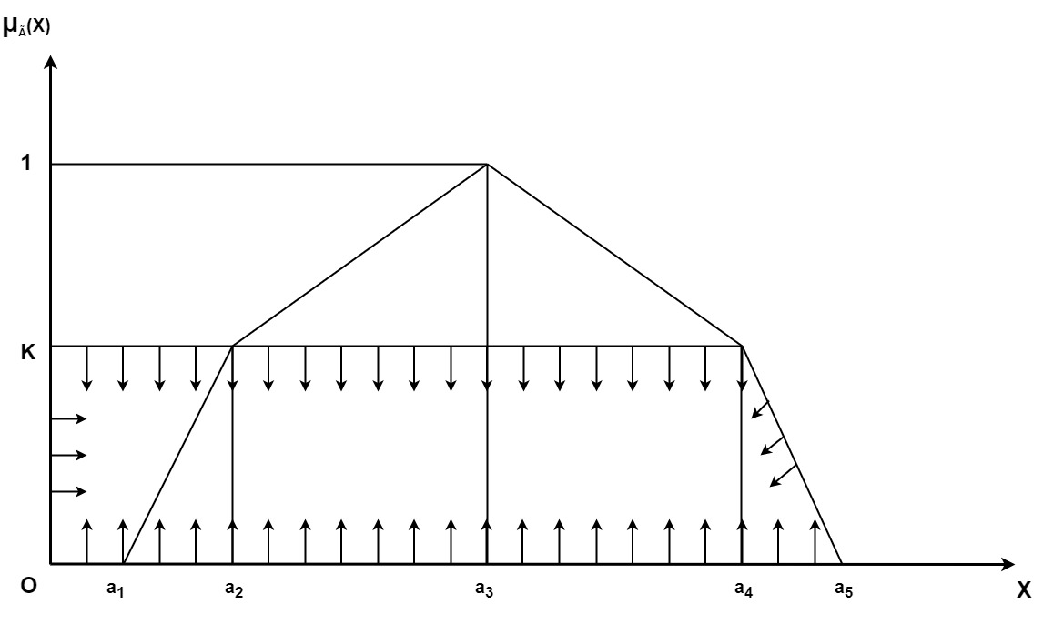
Table 3. Defuzzified pay-off matrix game.
This table is shown in the PDF version of the article.
Table 4. First step of dominance property.
This table is shown in the PDF version of the article.
Now each element of average of strategies Y3 and Y4 of player B are less than or
equal to the corresponding elements of strategy Y2 of player B. Therefore on deleting
the column of strategy Y2 by dominance property, we obtain a new modified matrix
game as Table (6).
Again each element of strategy X2 of player A is less than or equal to the corresponding
elements of the average of strategies X3 and X4 of player A. Therefore on deleting the
row of strategy X2 by dominance property, we obtain a new improved matrix game
as Table (7).
2 1 2 1 8
Which are A 0 is, 0 a,2× , 2 matrix and B game 0, 0, without , respectively and the value of game is saddle point, so the strategy of both.the players
3 3 3 3 3 Example 2. Consider a fuzzy matrix game for two different players A and B whose pay-offs are linear pentagonal fuzzy numbers with symmetry as follows:
Table 5. Second step of dominance property.
This table is shown in the PDF version of the article.
Table 6. Third step of dominance property.
This table is shown in the PDF version of the article.
Table 7. Fourth step of dominance property.
This table is shown in the PDF version of the article.
Now using the mean of α-cut method as defuzzification defined by equation (32) for the linear pentagonal fuzzy number to convert the given fuzzy pay-off matrix game
as Table (8) into the crisp matrix game defined by the Table (9), as follows:
Table 8. Defuzzified pay-off matrix game.
This table is shown in the PDF version of the article.
Since the above crisp matrix game defined by Table (8) has no saddle point, there-
fore according to the dominance property in matrix games, strategy X1 of player A
can be dominated by strategy X3 of player A. Hence we have a modified matrix game
defined by Table (9).
Table 9. First step of dominance property.
This table is shown in the PDF version of the article.
Again we have that all the elements of strategy Y1 are greater than or equal to the
corresponding elements of strategy Y3 for player B. Therefore strategy Y1 dominates
strategy Y3 and so we can delete the strategy column Y1 for new improved matrix
game as Table (10).
Table 10 Second step of dominance property.
Strategy Y2 Y3 Y4
X2 5 3 5 X3 3 5 0 X4 4 0 9
Further the matrix game as Table (10) can not be reduced by dominance rule. There-
fore by applying the linear programming approach for matrix game, we have
For Player A
max v such that 5x1 + 3x2 + 4x3 ≥ v 3x1 + 5x2 + 0x3 ≥ v 5x1 + 0x2 + 9x3 ≥ v x + x + x = 1 1 2 3 and x1, x2, x3, v ≥ 0.
and
For Player B min w
such that 5y + 3y + 5y ≤ w 1 2 3 3y1 + 5y2 + 0y3 ≤ w 4y + 0y + 9y ≤ w 1 2 3 y1 + y2 + y3 = 1 and y , y , y , w ≥ 0.
1 2 3
Where v, w are the minimum expected gain and maximum expected loss for player A
and B respectively. The above linear programming problems for player A and player B as x y can be written in the following manner by assuming = Ri, = Sj for i, j = 1, 2, 3 For Player A v w min R1 + R2 + R3
such that
5. R1 + 3R2 + 4R3 ≥ 1
3R1 + 5R2 + 0R3 ≥ 1 5R1 + 0R2 + 9R3 ≥ 1
and R1, R2, R3 ≥ 0.
and
For Player B max S1 + S2 + S3
such that 5S + 3S + 5S ≤ 1
1 2 3
3. S1 + 5S2 + 0S3 ≤ 1
4S + 0S + 9S ≤ 1 1 2 3 and S1, S2, S3 ≥ 0.
On solving the above linear programming problems by the classical simplex method, 0.28. So the optimal strategy of both the players A and B are A (0, 0.1 71429, 0.28571 1, 0) we obtain R1 = 0.2; R2 = 0.08; R3 = 0; S1 = 0; S2 = 0.2; S3 = 0.08; = 0.28 and = and B (0, 0, 0.71429, 0.28571) respectively and the value of game is 3.57143. In [6] the
9 5 9 5
optimal strategies of the players A 0, 0, , and B 0, 0, , and the value of
14 14 14 14
45 were evaluated.
game 14
Example 3. Consider a fuzzy matrix game for two different players A and B whose pay-offs are linear pentagonal fuzzy numbers with symmetry as follows:
Now using the mean of α- cut method as defuzzification defined by Eq. (32) for the linear pentagonal fuzzy number to convert the given fuzzy pay-off matrix game
as Table (11) into the crisp matrix game defined by the Table (13), as follows: Since the above crisp matrix game defined by Table (11) has no saddle point,
Table 11. Defuzzified pay-off matrix game.
This table is shown in the PDF version of the article.
Table 12. Defuzzified pay-off matrix game obtained by [6].
This table is shown in the PDF version of the article.
therefore according to the dominance property in matrix games, strategy X1 can be
dominated by strategy X3 of player A. Hence we have a modified matrix game defined
by Table (13).
Table 13. First step of dominance property.
This table is shown in the PDF version of the article.
Again we have that all the elements of strategy Y1 are equal to the corresponding
elements of strategy Y3 for player B. Therefore either strategy Y1 or strategy Y3 for
player B can be dominated by each other. Here we delete the strategy Y1 for the new,
improved matrix game as Table (14).
Now each element of the average of strategies Y3 and Y4 of player B are less than or
equal to the corresponding elements of strategy Y2 of player B. Therefore on deleting
the column strategy Y2 by dominance property, we obtain a newly modified matrix
game defined by the following Table (15) as Further the matrix game as Table (14) can not be reduced by dominance rule.
Table 14. Second step of dominance property.
This table is shown in the PDF version of the article.
Table 15. Third step of dominance property.
This table is shown in the PDF version of the article.
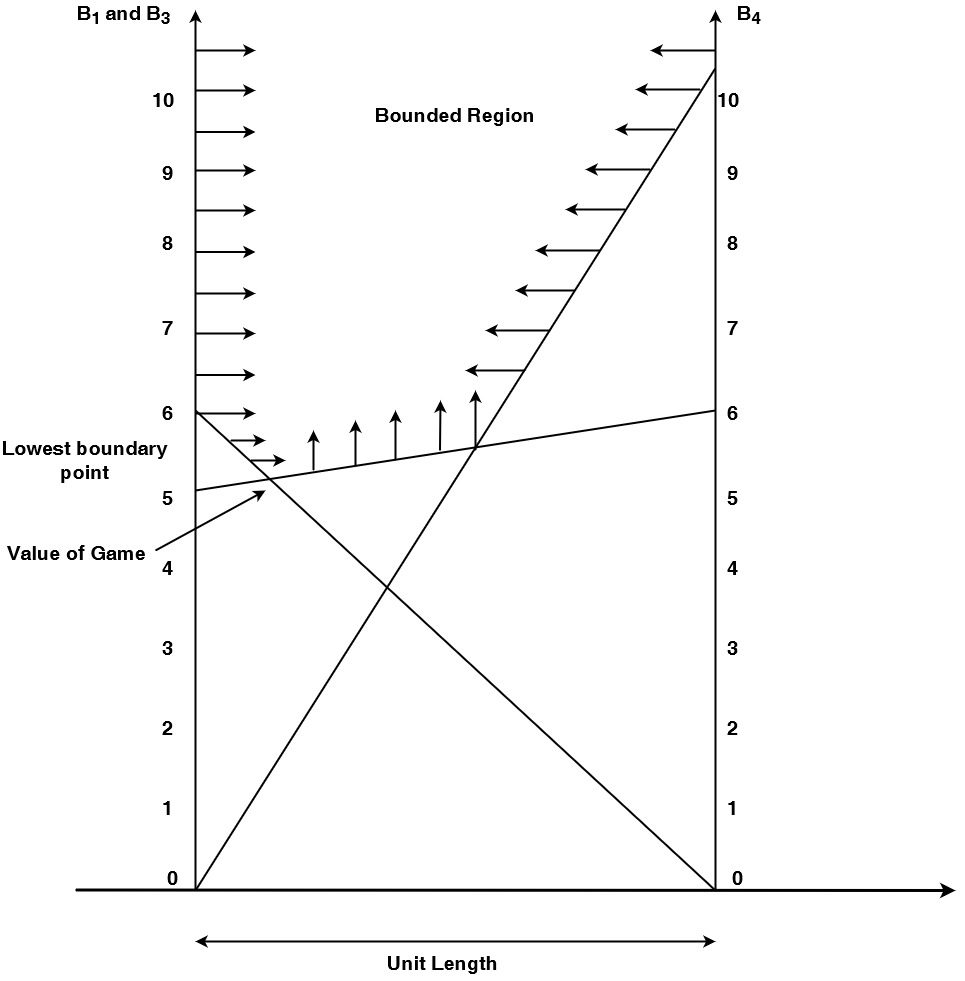
Therefore by applying the graphical approach for m × 2 matrix game according as
Table (15) given by Figure 17.
Hence it is clear that the lowest boundary point P on the bounded region will give
the smallest expected loss to the minimizing player (playerB). So the best strategy
for player A are those which pass through the point P. Therefore we can write the
matrix game as given by the Table (15) in a 2 × 2 matrix game defined by the Table
(16) as follows:
Table 16. Fourth step of dominance using graphical method.
This table is shown in the PDF version of the article.
The above 2 × 2 matrix game is without saddle point, so the strategy of both the
6 1 6 1 36
players are A 0, , , 0 and B 0, 0, , respectively and the value of game is . In
7 7 7 7 7 5 3 5 3
[6] the optimal strategies of the players A 0, 0, , , B 0, 0, , and the value of
8 8 8 8
the game were evaluated.
Remark 1. If we delete the strategy Y3 for new improved matrix game as second step
of dominance property and further on going in a similar manner, we obtain the best
1 6 1
6 , , 0 and B , 0, 0, respectively and the strategy for player A and B as A 0, 7 7 7 7 value of game is .
5.1 Comparative Study of Proposed Defuzzification Techniques
by Numerical Examples
In this section we compared all the proposed defuzzification techniques numerically
for matrix game problems assigned by [6] and investigate that I. The strategy of the game players remains unchanged in realistic game problems.
II. Centroid method and mean of α-cut method provides the same results.
III. Value of the matrix game obtained by removal of region method is the half of the
game value obtained by other remaining proposed methods.
6. Conclusion
This research paper has systematically explored and elucidated a range of mathemat-
ical concepts central to the pentagonal fuzzy numbers. The investigation developed
various concepts, including distinct representations, intrinsic properties, α-cuts, and defuzzification methodologies. The application of both linear and non-linear member-ship functions in a symmetric fashion has been rigorously examined, contributing to a comprehensive understanding of the subject. The incorporation of numerical exam-ples drawn from matrix game problems, as originally provided by [6], has added depth and context to the discourse. The introduction and analysis of novel defuzzification techniques for pentagonal fuzzy numbers have provided valuable insights into optimal strategies for players, as well as the determination of game values—parameters of sub-stantial significance within real-world gaming scenarios. This paper offers a stepping stone for further scholarly inquiries into the field of pentagonal fuzzy numbers across diverse real-life problem domains. By shedding light on the representation, defuzzifica-tion, and their applications within the context of game theory, this research develops the way for continued exploration and innovative utilization of pentagonal fuzzy num-bers in addressing complex phenomena. Researchers are encouraged to build upon this foundation, unraveling the potential of pentagonal fuzzy numbers as a powerful tool to handle the real-world challenges.
Acknowledgments
The authors would like to express their appreciation to all individuals whose valuable comments and suggestions contributed to the improvement of this research.
Funding
The authors declare that no financial support, grant, or sponsorship was received for conducting this study.
Data Availability
The data used and analyzed during the current study are available from the corre-sponding author upon reasonable request.
Figures
References
- [1] Abbasbandy, S., & Hajjari, T. (2009). A new approach for ranking of trapezoidal fuzzy numbers. Computers & mathematics with applications, 57(3), 413-419. https://doi.org/10.1016/j.camwa.2008.10.090
- [2] Asady, B., & Zendehnam, A. (2007). Ranking fuzzy numbers by distance mini-mization. Applied mathematical modelling, 31(11), 2589- 2598.https://doi.org/10.1016/j.apm.2006.10.018
- [3] Atanassov, K. T. (1999). Intuitionistic fuzzy sets. In Intuitionistic fuzzy sets: theory and applications (pp. 1-137). Heidelberg: Physica-Verlag HD. https://doi.org/10.1007/978-3-7908-1870-3_1
- [4] Atanassov, K. T. (1986) ‘Intuitionistic fuzzy sets’, Fuzzy Sets Syst, 20(1), 87–96.
- [5] Buckley, J. J. (1988). Possibilistic linear programming with triangular fuzzy numbers. Fuzzy sets and Systems, 26(1), 135-138. https://doi.org/10.1016/0165-0114 (88)90013-9
- [6] Chakraborty, A., Mondal, S. P., Alam, S., Ahmadian, A., Senu, N., De, D., & Salahshour, S. (2019). The pentagonal fuzzy number: its different representa-tions, properties, ranking, defuzzification and application in game problems. Symmetry, 11(2), 248.
- [7] Chen, S. M. (2011). Analyzing fuzzy risk based on a new fuzzy ranking method between generalized fuzzy numbers. Expert Systems with Applications, 38(3), 2163- 2171. https://doi.org/10.1016/j.eswa.2010.08.002
- [8] Cheng, C. H. (1998). A new approach for ranking fuzzy numbers by distance method. Fuzzy sets and systems, 95(3), 307-317. https://doi.org/10.1016/S0165-0114 (96)00272-2
- [9] Chou, C. C. (2003). The canonical representation of multiplication operation on triangular fuzzy numbers. Computers & Mathematics with Applications, 45(10-11), 1601-1610. https://doi.org/10.1016/S0898-1221(03)00139-1
- [10] Chutia, R., & Chutia, B. (2017). A new method of ranking parametric form of fuzzy numbers using value and ambiguity. Applied soft computing, 52, 1154- 1168. https://doi.org/10.1016/j.asoc.2016.09.013
- [11] Dubois, D., & Prade, H. (1978). Operations on fuzzy numbers. International jour-nal of systems science, 9(6), 613-626. https://doi.org/10.1080/00207727808941724
- [12] Dubois, D., & Prade, H. (Eds.). (2012). Fundamentals of fuzzy sets (Vol. 7). Springer Science & Business Media. https://link.springer.com/book/10.1007/978-1-4615 -4429-6
- [13] Garg, H. (2018). Some arithmetic operations on the generalized sigmoidal fuzzy numbers and its application. Granular computing, 3(1), 9-25.. https://doi.org/10.1007/s41066-017-0052-7
- [14] Heilpern, S. (1997). Representation and application of fuzzy numbers. Fuzzy sets and systems, 91(2), 259-268. https://doi.org/10.1016/S0165-0114(97)00146-2
- [15] Kaur, A., & Kumar, A. (2012). A new approach for solving fuzzy transportation prob-lems using ´ generalized trapezoidal fuzzy numbers. Applied soft computing, 12(3), 1201- Kosiń ski, W., Prokopowicz, P., & Ś lę zak, D. (2003). Ordered fuzzy numbers. 1213. https://doi.org/10.1016/j.asoc.2011.10.014 bulletin of the polish academy of sciences, 51(3), 327-338.
- [16] http://users.pja.edu.pl/~wkos/11-KOSIN.PDF
- [17] Massanet, S., Riera, J. V., Torrens, J., & Herrera-Viedma, E. (2014). A new lin-guistic computational model based on discrete fuzzy numbers for computing with words. Information sciences, 258, 277-290. https://doi.org/10.1016/j.ins.2013.06.055
- [18] Nayagam, V. L. G., Jeevaraj, S., & Sivaraman, G. (2016). Complete ranking of intuitionistic fuzzy numbers. Fuzzy Information and engineering, 8(2), 237-254. https://doi.org/10.1016/j.fiae.2016.06.007
- [19] Nehi, H. M. (2010). A new ranking method for intuitionistic fuzzy numbers. International journal of fuzzy systems, 12(1).https://www.researchgate.net/publica-tion/279900044_A_New_Ranking_Method_for_Intuitionistic_Fuzzy_Numbers
- [20] Panda, A., & Pal, M. (2015). A study on pentagonal fuzzy number and its corre-sponding matrices. Pacific science review B: humanities and social sciences, 1(3), 131-139. https://doi.org/10.1016/j.psrb.2016.08.001
- [21] Qiu, D., & Zhang, W. (2013). Symmetric fuzzy numbers and additive equivalence of fuzzy numbers. Soft computing, 17(8), 1471-1477.https://doi.org/10.1007/s00500-013-1000-3
- [22] Rouhparvar, H., & Panahi, A. (2015). A new definition for defuzzification of gen-eralized fuzzy numbers and its application. Applied Soft Computing, 30, 577-584. https://doi.org/10.1016/j.asoc.2015.01.053
- [23] Seresht, N. G., & Fayek, A. R. (2019). Computational method for fuzzy arith-metiac operations on triangular fuzzy numbers by extension principle. International journal of approximate reasoning, 106, 172-193. https://doi.org/10.1016/j.ijar.2019.01.005
- [24] Smarandache, F. (1999). A unifying field in logics neutrosophy: neutrosophic probability. Set and Logic.
- [25] Wang, Y. M., Yang, J. B., Xu, D. L., & Chin, K. S. (2006). On the centroids of fuzzy numbers. Fuzzy sets and systems, 157(7), 919-926. https://doi.org/10.1016/j.fss.2005.11.006
- [26] Xu, Z., Shang, S., Qian, W., & Shu, W. (2010). A method for fuzzy risk analysis based on the new similarity of trapezoidal fuzzy numbers. Expert Systems with Applications, 37(3), 1920-1927. https://doi.org/10.1016/j.eswa.2009.07.015
- [27] Yager, R. R. (1986). On the theory of bags. International journal of general system, 13(1), 23-37. https://doi.org/10.1080/03081078608934952
- [28] Zad´eh, L.A. (1965) ‘Fuzzy sets’, Information and control, 8(3), 338–353.
- [29] Zadeh, L. A. (1975). The concept of a linguistic variable and its application to ap-proximate reasoning—I. Information sciences, 8(3), 199-249. https://doi.org/10.1016/0020-0255(75)90036-5