
Integer Programming Problems with Fermatean Fuzzy Parameters Using NAZ-Cut
Abstract
Integer Programming Problems (IPPs) play a critical role in solving real-world optimization scenarios where decision variables must be integers, such as in scheduling, logistics, and resource allocation. Traditional methods like Branch and Bound and Cutting Plane techniques have been widely used for solving such problems. In 2003, Bari and Ahmad introduced the NAZ-cut method, a straightforward and computationally efficient approach to solving IPPs by systematically reducing the feasible solution space through the addition of specific constraints. This paper presents an enhanced NAZ-cut framework for solving IPPs, particularly in the context of Fermatean fuzzy environments, where uncertainty in parameters is modeled using Fermatean fuzzy sets. A new approach is proposed to minimize computational effort by excluding specific integer candidate solutions based on a well-defined criterion. A supporting theorem is provided to justify this exclusion, ensuring that only feasible and potentially optimal points are considered. The method is demonstrated through a numerical example, highlighting the effectiveness of the proposed strategy in simplifying the search process and improving computational efficiency.
Keywords:NAZ cutFermatean fuzzy paramatersBranch and bound methodsCutting plane methodsOptimization
1. Introduction
Most of the real-life problems are such that they require integer solutions and non-integral solutions do not create any sense for such problems. For example, a car manufacturing unit cannot manufacture cars in fractions, similar to problems like the distribution of goods; scheduling, machine sequencing, etc. The solution should have an integer value. Other problems include planning problems such as capital budgeting, facility location, portfolio analysis, and design problems such as communication and transport network design, circuit design, and the design of automated production systems. Integer programming (IP) is a mathematical optimization technique used to find the best solution to a problem within a defined set of constraints, where some or all of the decision variables are required to take on integer values [1], [2]. This characteristic distinguishes IP from Linear Programming (LP), which allows decision variables to take any value within a continuous range. The integrality constraint in IP is crucial in applications where variables represent discrete items, such as the number of products to produce, people to assign, or vehicles to route [3], [4].
IPP can be classified into different types based on the nature of the integer constraints [5]. Pure Integer Programming Problems (IPPs) involve decision variables that are all integers, while Mixed-Integer Programming (MIP) problems have both integer and continuous variables [6], [7]. Another variant, Binary Integer Programming (BIP), restricts some or all decision variables to binary values (0 or 1), making it particularly useful for modeling yes/no decisions or selection problems [6]. The formulation of an IP problem typically involves three components: an objective function, a set of decision variables, and a set of constraints. The objective function represents the goal of the optimization, such as maximizing profit or minimizing cost. The constraints define the limitations or requirements that the solution must satisfy, such as resource availability or capacity limits. IP models are widely used in various fields, including operations research, logistics, finance, and manufacturing, due to their ability to model real-world situations involving discrete choices and logical conditions [8], [9].
In recent years, modeling uncertainty in real-world optimization problems has gained significant attention. Classical IP assumes that all parameters are known with certainty; however, in practice, many problems involve vagueness, imprecision, or incomplete information. To address this, fuzzy set theory has been applied to mathematical programming. Among the various fuzzy models, Fermatean fuzzy sets—an extension of Intuitionistic and Pythagorean fuzzy sets—offer a more flexible and expressive framework for handling uncertainty. Incorporating Fermatean fuzzy parameters into IPPs allows decision-makers to capture a higher degree of hesitation and uncertainty in the problem data. This paper extends the NAZ-cut approach to handle IPPs with Fermatean fuzzy parameters, offering a novel solution technique that is both computationally efficient and robust under fuzzy uncertainty.
Despite its widespread applicability, solving IP problems can be computationally challenging. Unlike LP problems, which can be efficiently solved using polynomial-time algorithms like the Simplex method or interior-point methods [10], IP problems are often NP-hard [11]. This means that as the problem size increases, the time required to find an optimal solution can grow exponentially. As a result, exact algorithms like branch and bound [12], cutting planes method [13], and branch and cut are employed, though they may be computationally intensive [14]. In practice, heuristic and metaheuristic methods, such as genetic algorithms, simulated annealing, and tabu search, are frequently used to find near-optimal solutions within a reasonable time frame. A mathematical programming problem (MPP) with integer restrictions is termed an IPP and the mathematical formulation of IPP with fermatean fuzzy parameters is given as follows:
max Z ̃ = g (x ̃ , x ̃ , . . . , x ̃ ),
0 1 2 n
s.t.
g (x ̃ , x ̃ , . . . , x ̃ ) ≤ or = or ≥ b ̃ , i = 1, 2, … , m, (1)
i 1 2 n i
x ̃j ≥ 0, j ∈ N ≡ {1 ,2 , . . . , n}, x ̃j integer.
If all x ̃j are integer, i.e. all the variables x ̃j are restricted to have integer values, the problem is called a pure IPP. Otherwise, if some and not all x ̃j are integer then it is a mixed IPP. As we have seen IPP is very useful, particularly in real-life problems. So, it was very important to develop some methods to solve IPPs [15]. The crisp mathematical model is represented as follows:
max Z ̃ = g (S(x ̃ , x ̃ , . . . , x ̃ )),
0 1 2 n
s.t.
g (S(x ̃ , x ̃ , . . . , x ̃ )) ≤ or = or ≥ S(b ̃ ), i = 1, 2, … , m, (2)
i 1 2 n i
S(x ̃j) ≥ 0, j ∈ N ≡ {1 ,2 , . . . , n}, S(x ̃j) integer.
Mathematical programming approaches to solve IPPs are very important in today’s world. Dantzig et al. [16] and Markowitz and Manne [17] were the first whose works drew the attention of researchers to visualize the importance of solving linear programs in integers. Gomory [18], [19] developed the first finite cutting algorithm for the pure IPP. Ben-Israel and Charnes [20] introduced the primal algorithm of the IPP with various variables. After that, Young [21] developed a finite primal algorithm in the field of IPP and mathematical programming problems. A method using Benders [22] partitioning scheme was devised by Harris [23] for MIP. Trotter and Shetty [24] proposed an algorithm for the bounded variable pure IPPs. Granot and Granot [25] constructed a new cutting plane algorithm for solving integer fractional programming and mixed integer fractional programming problems using Charnes and Cooper [20]. approach for solving the integer continuous fractional programs.
Then came the concept of branch and bound in mathematical programming. Land and Doig [26] developed the branch and bound algorithm first time for solving the pure and mixed IPP. Bertier and Roy [27] later, presented a general theory for branching and bounding. Balas [28] restated their theory in a far simpler form which Mitten [29] generalized and extended slightly. A lot more work has been done on integer and mixed IPPs. Few of them represent a lot of work in the field of IPPs (Guignard and Spielberg [30], Lenstra [31], Hoffman and Padberg [32], Savelsberg [33], Balas et al. [34], Weismantel [35]). Some recent works to solve the integer pure and mix programming problem using different approaches (Kesavana et al., [36], Frangioni and Gentile [37], Vyve and Wolsey [38], Lay and Jacobson [39], Cadoux [40], Basu et. al. [41], Jansen and Rohwedder [42], Hooker [43], Goswami [44].
2. Formulation of the Problem
The basic definitions of the Farmatean fuzzy programming, which are used in our proposed work, which is given below:
Definition 1. According to [45] Farmatean fuzzy sets: A Farmatean Fuzzy Sets (FFSs) can be represented as ℱ ̃ = {〈ω, α ̃(ω), β ̃(ω): ω ∈ X 〉}, where αℱ ̃(ω): X → [0,1] is the degree of satisfaction, and βℱ ̃(ω): X → [0,1] is the degree of dissatisfaction, including the conditions.
3 3 ̃
0 ≤ αℱ ̃(ω) + βℱ ̃(ω) ≤ 1 for all ω ∈ X . For any FFSs ℱ and ω ∈ X,
3 3 3
σ ̃(ω) = √1 − (α ̃(ω)) − (β ̃(ω)) is identified as the degree of indeterminacy of ω ∈ X to ℱ ̃.The set ℱ ̃ =
ℱ ℱ ℱ
{〈ω, α ̃(ω), β ̃(ω): ω ∈ X 〉} is denotes as ℱ ̃ = 〈α ̃, β ̃〉.”
ℱ ℱ ℱ ℱ
Definition 2. Let ℱ ̃ = 〈α ̃, β ̃〉, ℱ ̃ = 〈α ̃ , β ̃ 〉, and ℱ ̃ = 〈α ̃ , β ̃ 〉 be three FFSs on the universal set X, and
ℱ ℱ 1 ℱ1 ℱ1 2 ℱ2 ℱ2
ζ > 0 be any scalar, then arithmetic operations of FFSs is as follows with numerical examples.
̃ ̃ 3 3 3 3 ℱ1 ⊕ ℱ2 = (√αℱ ̃ + αℱ ̃ − αℱ ̃ αℱ ̃ , βℱ ̃ βℱ ̃ ).
Let ℱ ̃ = 〈0.4, 0.7〉 , ℱ ̃ = 〈0.8, 0.6〉 and ℱ ̃ = 〈0.2, 0.9〉 be three FFSs and ζ = 2 be any scalar quantity. Then,
ℱ ̃ ⊕ ℱ ̃ = 〈0.8, 0.6〉 ⊕ 〈0.2, 0.9〉 = (0.8020, 0.54).
3 3 3 3 3
ℱ ̃ ⊗ ℱ ̃ = (α α , √β + β − β β ),
1 2 ℱ ̃ ℱ ̃ ℱ ̃ ℱ ̃ ℱ ̃ ℱ ̃
ℱ ̃ ⊗ ℱ ̃ = 〈0.8, 0.6〉 ⊕ 〈0.2, 0.9〉 = (0.16, 0.923).
̃ √ ( 3)ζ ζ ⊙ ℱ = ( 1 − 1 − αℱ ̃ , βℱ ̃ ),
ζ ⊙ ℱ ̃ = 2 ⊙ 〈0.4, 0.7〉 = (0.498, 0.49).
ζ ζ √ 3 ℱ ̃ = (α , 1 − (1 − β ) ).
ℱ ̃ ℱ ̃
̃ ζ 2 ℱ = 〈0.4, 0.7〉 = (0.064,0.828).
Definition 3. Let ℱ ̃ = 〈α ̃, β ̃〉, ℱ ̃ = 〈α ̃ , β ̃ 〉, and ℱ ̃ = 〈α ̃ , β ̃ 〉 be three FFSs on the universal set X, and
ℱ ℱ 1 ℱ1 ℱ1 2 ℱ2 ℱ2
ζ > 0 be any scalar, then their arithmetic operations of FFS define as follows:
ℱ ̃ ⋃ℱ ̃ = (max{α , α } , min{β , β }),
1 2 ℱ ̃ ℱ ̃ ℱ ̃ ℱ ̃
1 2 1 2
ℱ ̃ ⋃ℱ ̃ = (max{〈0.8, 0.6〉} , min{〈0.2, 0.9〉}) = (0.8, 0.2).
ℱ ̃ ⋂ℱ ̃ = (min{α , α } , max{β , β }).
1 2 ℱ ̃ ℱ ̃ ℱ ̃ ℱ ̃
1 2 1 2
ℱ ̃ ⋂ℱ ̃ = (min{〈0.8, 0.6〉} , max{〈0.2, 0.9〉}) = (0.2, 0.6).
ℱ = (βℱ ̃ , αℱ ̃).
̃ c c ℱ = 〈0.4, 0.7〉 = (0.7,0.4).
̃ ̃ ̃ ∗ ̃
Theorem 1. Let ℱ be a FFSs ℱ = 〈αℱ ̃, βℱ ̃〉 then the score function ℱ represented simply proceeds: Sℱ ̃ (ℱ ) =
1 3 3
(1 + αℱ ̃ − βℱ ̃ ). (min(αℱ ̃, βℱ ̃)).
̃ ∗ ̃
Property 1: Consider a FFSs ℱ = 〈αℱ ̃, βℱ ̃〉, then Sℱ ̃ (ℱ ) ∈ [0,1].
Proof: According to the ortho-pair definition, αℱ ̃, βℱ ̃ ∈ [0,1]. Then, min(αℱ ̃, βℱ ̃) ∈ [0,1], and also αℱ ̃ ≥ o,
3 3 3
βℱ ̃ ≥ 0, αℱ ̃ ≤ 1, and βℱ ̃ ≤ 1.
⇒ 1 − βℱ ̃ ≥ 0, ⇒ 1 + αℱ ̃ − βℱ ̃ ≥ 0, ∴ (1 + αℱ ̃ − βℱ ̃ ). (min(αℱ ̃, βℱ ̃)) ≥ 0.
Again αℱ ̃ − βℱ ̃ ≤ 1, add one both sides.
3 3 3
⇒ 1 + αℱ ̃ − βℱ ̃ ≤ 2 (∵ αℱ ̃ ≥ 0),
⇒ (1 + αℱ ̃ − βℱ ̃ ). (min(αℱ ̃, βℱ ̃ )) ≤ 1 (∵ min(αℱ ̃ , βℱ ̃ ) ≤ 1).
Hence, Sℱ ̃ (ℱ ) ∈ [0,1].
̃ ̃ ̃ ∗ ̃
Theorem 2. Let ℱ be a FFSs ℱ = 〈αℱ ̃, βℱ ̃〉 then the NFFSF ℱ1d represented simply as follows: Sℱ ̃ (ℱ1d) = (1 + αℱ ̃ − βℱ ̃). (min(αℱ ̃, βℱ ̃)) .
̃ ∗ ̃
Property 1: Consider a FFSs ℱ = 〈αℱ ̃, βℱ ̃〉, then Sℱ ̃ (ℱ1d) ∈ [0,1].
Proof: According to the ortho-pair definition, αℱ ̃, βℱ ̃ ∈ [0,1]. Then, min(αℱ ̃, βℱ ̃) ∈ [0,1], and also αℱ ̃ ≥ o, βℱ ̃ ≥ 0, αℱ ̃ ≤ 1, and βℱ ̃ ≤ 1.
⇒ 1 − βℱ ̃ ≥ 0, ⇒ 1 + αℱ ̃ − βℱ ̃ ≥ 0,∴ (1 + αℱ ̃ − βℱ ̃). (min(αℱ ̃ , βℱ ̃ )) ≥ 0.
Again, αℱ ̃ ≤ 1, and βℱ ̃ ≤ 1, αℱ ̃ − βℱ ̃ ≤ 1, add one both sides.
⇒ 1 + αℱ ̃ − βℱ ̃ ≤ 2 ⇒ (min(αℱ ̃ , βℱ ̃ ) ≤ 1) ⇒ (min(αℱ ̃ , βℱ ̃ )) ≤ 1,
⇒ (1 + αℱ ̃ − βℱ ̃ ). (min(αℱ ̃, βℱ ̃ )) ≤ 1 (∵ (min(αℱ ̃, βℱ ̃ )) ≤ 1).
Hence, Sℱ ̃ (ℱ1d) ∈ [0,1].
Theorem 3. Let ℱ ̃ be a FFSs ℱ ̃ = 〈α ̃, β ̃〉 then the Type 1 score function ℱ ̃ represented as follows:
ℱ ℱ 1 ∗ 1 2 2
Type-1 Fermatean fuzzy score function S (ℱ ̃ ) = (1 + α − β ).
ℱ ̃ 11 ℱ ̃ ℱ ̃ 2 2 2 2
According to the ortho-pair definition, α ̃, β ̃ ∈ [0,1], and α ̃ ≥ o, β ̃ ≥ 0, α ̃ ≤ 1, and β ̃ ≤ 1.
ℱ ℱ ℱ ℱ ℱ ℱ
⇒ 1 − βℱ ̃ ≥ 0, ⇒ 1 + αℱ ̃ − βℱ ̃ ≥ 0 ∴ (1 + αℱ ̃ − βℱ ̃ ) ≥ 0.
Now, again, αℱ ̃ − βℱ ̃ ≤ 1, add on both sides.
2 2 2
⇒ 1 + αℱ ̃ − βℱ ̃ ≥ 2 (∵ αℱ ̃ ≥ 0),
⇒ (1 + αℱ ̃ − βℱ ̃ ) ≥ (∵ 〈αℱ ̃, βℱ ̃ 〉 ≤ 1).
Hence, Sℱ ̃ (ℱ11) ∈ [0,1]. Similarly,
∗ 1 3 3
Type-2 Fermatean fuzzy score function S ̃ (ℱ ̃ ) = (1 + 2α ̃ − β ̃ ).
ℱ 12 ℱ ℱ ∗ 1 2 2
Type-3 Fermatean fuzzy score function S ̃ (ℱ ̃ ) = (1 + α ̃ − β ̃ ). |α ̃ − β ̃|.
ℱ 13 ℱ ℱ ℱ ℱ
Let ℱ ̃ = 〈α ̃ , β ̃ 〉, and ℱ ̃ = 〈α ̃ , β ̃ 〉 be two FFSs, then the following operations will be satisfied:
1 ℱ1 ℱ1 2 ℱ2 ℱ2
∗ ̃ ∗ ̃ ̃ ̃ ̃ ̃ Sℱ ̃ (ℱ1 ) ≥ Sℱ ̃ (ℱ2 ) with Aℱ ̃(ℱ1) > Aℱ ̃(ℱ2) iff ℱ1 > ℱ2.
∗ ̃ ∗ ̃ ̃ ̃ ̃ ̃ Sℱ ̃ (ℱ1 ) ≤ Sℱ ̃ (ℱ2 ) with Aℱ ̃(ℱ1) < Aℱ ̃(ℱ2) iff ℱ1 < ℱ2.
∗ ̃ ∗ ̃ ̃ ̃ ̃ ̃ Sℱ ̃ (ℱ1 ) = Sℱ ̃ (ℱ2 ) with Aℱ ̃(ℱ1) = Aℱ ̃(ℱ2) iff ℱ1 = ℱ2.
Consider the following Pure Integer Programming Problem (PIPP)
Max Z = c x
s.t.
Am×n x ≤ b,
x ≥ 0.
Where c are the fermatean fuzzy coefficients representing the contribution of each variable x to the fermaten fuzzy objective function, x = (x1,x2 … xn), A is m × n matrix of coefficient, and b is an m − dimensional vector of constants.
Let us consider that Linear Programming Problem (LPP), neglecting the integer restrictions on the variables as Linear Programming Relaxation (LPR). First, we solve the LPR problem. Let the solution obtained be x and is all integer. It implies that the problem is solved. Now consider the case when the solution is not an
th ∗ k ∗ k
integer and let the k component of x be x = ak. The nearest integer values to x are represented as follows:
k ∗ k ∗ ∗
x = [a ] and x = [a ] + 1 = 〈a 〉, for k = 1, 2, … , n. (6)
1 k 2 k k where [t] is the largest integer less than or equal to t and 〈t〉 is the smallest integer greater than or equal to t. With such bifurcations, we can find all the 2 integer points in the surrounding of the noninteger x solution (e.g. in case of 2 variable problems if x = (2.2, 3.6), then these will be 2 = 4 integer points viz. (2, 3), (2, 4), (3,3) and (3,4) around x . Let us denote the set of indices of these 2 points by T also, the
∗ ∗ ∗
objective value at x is z . Thus, the objective function level plane at x is given by
cx = z . (5)
Then we find the perpendicular distance di from the surrounding points, to the objective function level plane by using the formula given by Dantzig [16].
z − cxi di = , i ∈ T.
√∑ c
j=1 j
where xi is an integer point around x .
But, here we are finding the difference by this formulae di = z − cxi , i ∈ T, given by Adhami and Rabbani [46] where they have taken the difference between objective function values at surrounding integer. The next step is to search the integer point xi , which has a minimum distance from the objective hyperplane. The negative distance and the distances from the infeasible points should be omitted. We choose the minimum positive distance only from the feasible points.
o o o
Let S be a set of indices i ∈ T for which xi are feasible. Let xi = {xk │dk = min di}.Now, as we have to search for the feasible point xi which has a minimum positive difference from the objective function value. So, consider the two variable problem as (x1, x2), which is a non-integer and its surrounding integer points will
∗ ∗ ∗ ∗ ∗ ∗ ∗ ∗
be ( [x ], [x ] ), ( [x ], 〈x 〉), ( 〈x 〉, [x ] ) and (〈x1〉, 〈x2〉) and the notations have the same meaning described
∗ k ∗ k
above. Now, consider the case 〈x1〉 = x1, 〈x2〉 = x2. By using simple mathematics, we can say that di will
∗ k ∗ k ∗
always be negative for these values of xi for which ( x1 > x1 and x2 > x2). So, at this point, the distance will always be negative and we will always reject this point. Thus, for two-variable problems, we will have to search for 3 points. And this can be generalized for n − variable problems where we have to search for 2 − 1 points. Theorem 1. If each variable in the point of search is greater than its respective continuous optimal solution, then that point will always be neglected in NAZ- cut.
Proof: Let us consider a two-variable problem.
Min z = cx, A x ≤ b, x ≥ 0.
∗ ∗ ∗
Where x = (x1 , x2 ), A = (a1, a2) and x = (x1, x2 ) is the continuous optimal solution.
∗ k ∗ k ∗ ∗ k k
Also, 〈x1〉 = x1, 〈x2〉 = x2. Now, we have to show that (a1x1 + a2x2) − (a1x1 + a2x2)= negative quantity.
k ∗ k ∗
⇒ x1 > x1 ⇒ a1x1 > a1x1.
Similarly,
k ∗ k ∗
⇒ x2 > x2 ⇒ a2x2 > a2x2.
Now, we get
k k ∗ ∗
(a1x1 + a2x2) > (a1x1 + a2x2).
Therefore,
∗ ∗ k k
(a1x1 + a2x2) − (a1x1 + a2x2) = negative quantity
∗ ∗ ∗
We can extend it for n − variable problem which will be as follows: (a1x1 + a2x2 + ⋯ anxn) −
k k k
(a1x1 + a2x2 + ⋯ anxn) = negative quantity. Next, we proceed in the usual manner as we solve the NAZ cut. The procedure for solving the problem contains the following steps:
Step 1. Solve the LPP using the simplex or dual simplex method.
Step 2. If this solution is integer, stop. Otherwise, round off the non-integer solution to the nearest integers as described above in Eq. (3). Also, exclude the point whose value is greater than its respective continuous optimal solution (see Theorem 1).
Step 3. Find the minimum perpendicular distance from the integer point, which is inside the feasible region on the objective curve passing through the non-integer solution. Derive NAZ cut passing through this point and parallel to the objective function curve.
Step 4. Use the branch and bound or cutting plane method to find the integer optimum [47], [48].
3. Numerical Illustration
In this section, we consider a numerical example of the proposed problem.
Maximize Z = 2x1 + 3x2, subject to 5x1 + 2x2 ≤ 15, 3x1 + 5x2 ≤ 15, x1, x2 ≥ 0 and integer.
We will solve this problem considering it non-integer by using the simplex method and we get the following solution x1 = 2.37, x2 = 1.58, and z = 9.48. So, when we round off the obtained non-integer to the points as (2,2), (3,2), (3,1), and (2,1). From these points, we see that (3, 2) is that point in which both (3 > 2.37, 2 > 1.58). So we will reject this point here and will not consider it in further calculation. We are rejecting this point because we never consider negative distances and these types of points will always give negative distances. (see Theorem 1). Then, we calculate the perpendicular distance by this formula:
di = z − cxi .
Distance from the point (2, 2) is -0.52, Distance from the point (3, 1) is 0.48, Distance from the point (2, 1) is 2.48. We discard those points for which distances are negative and are outside the feasible region and check whether the constraints are satisfied for the points for which distance is positive. So, we get (2,1) as the required point. Furthermore, we derive the NAZ cut passing through the integer point (2,1) shown in Figure 1 below:
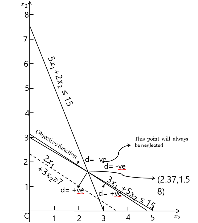
And then solving the new problem by using the branch and bound method (Daikin's Approach) as shown in
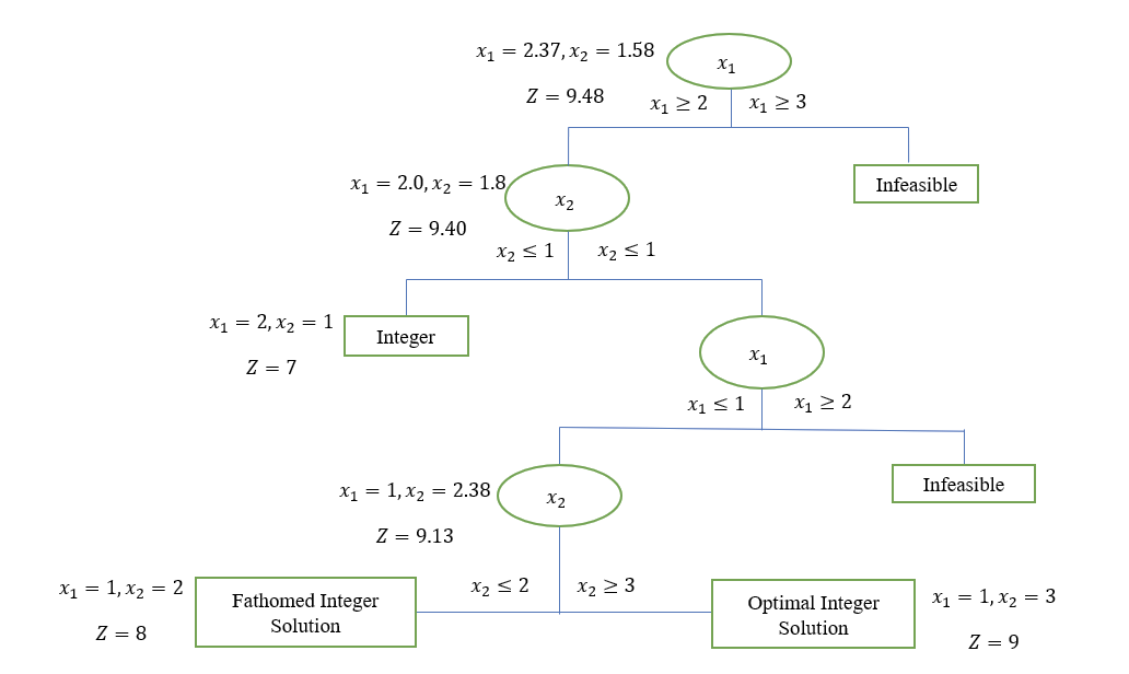
The compromise optimal solution is represented as follows: x1 = 0, x2 = 3 and z = 9.
4. Conclusion
In this study, we explored an enhanced approach to solving IPPs using the NAZ-cut method, particularly under the influence of Fermatean fuzzy parameters. The NAZ-cut technique, originally proposed by Bari and Ahmad, provides a simple yet powerful mechanism to reduce the feasible region of an IPP by introducing a constraint that systematically eliminates non-optimal regions. Our contribution lies in refining this method by identifying and excluding specific integer points that are guaranteed to yield negative distances from the objective function level plane, thereby reducing unnecessary computations. We established a supporting theorem to justify this exclusion, which simplifies the enumeration process without compromising the optimality of the solution. This theoretically grounded optimization not only enhances the computational efficiency of the NAZ-cut method but also makes it more scalable for higher-dimensional problems. Through a numerical example, we demonstrated how the proposed methodology can effectively identify the optimal integer solution while avoiding redundant calculations.
Furthermore, by incorporating Fermatean fuzzy parameters into the IP model, this work extends the applicability of the NAZ-cut method to problems characterized by uncertainty and imprecision. This integration broadens the relevance of our approach to real-world scenarios where exact parameter values are often unknown or imprecise. Future research may explore extending this framework to more complex multi-objective or dynamic environments, potentially integrating machine learning techniques to further enhance decision-making under fuzziness and constraint. In the present problem, we have discarded one point of enumeration out of 2 integer points as negative distances are not to be taken and this point will always give a negative distance, a theorem is also given in support of it. So, it will reduce the calculation as now the points for enumeration are 2 − 1 (n = number of variables) are points.
Data Availability
Required data is available in this manuscript.
Conflict of Interest
There are no competing interests to declare.
Consent for Publication
All authors have provided their consent for the publication of this manuscript
References
- [1] Antunes, C. H., Alves, M. J., & Clímaco, J. (2016). Multiobjective linear and integer programming. Cham, Switzerland: Springer. https://link.springer.com/book/10.1007/978-3-319-28746-1
- [2] Wolsey, L. A. (2020). Integer programming. John Wiley & Sons. https://www.wiley.com/en-us/Integer+Programming%2C+2nd+Edition-p-9781119606536
- [3] Paneque, M. P., Bierlaire, M., Gendron, B., & Azadeh, S. S. (2021). Integrating advanced discrete choice models in mixed integer linear optimization. Transportation research part b: methodological, 146, 26–49. https://doi.org/10.1016/j.trb.2021.02.003
- [4] Cornuéjols, G., Trick, M. A., & Saltzman, M. J. (1995). A tutorial on integer programming. https://cs.wmich.edu/gupta/teaching/cs6310/lectureNotes_cs6310/integer%20LP%20applications%20and%20so lutions%20from%20Clemson%201995.pdf
- [5] Papalexopoulos, T. P., Tjandraatmadja, C., Anderson, R., Vielma, J. P., & Belanger, D. (2022, June). Constrained discrete black-box optimization using mixed-integer programming. International Conference on Machine Learning (pp. 17295-17322). PMLR. https://proceedings.mlr.press/v162/papalexopoulos22a.html
- [6] Pisaruk, N. (2019). Mixed integer programming: Models and methods. Minsk: bsu. https://www.researchgate.net
- [7] Naderi, B., Ruiz, R., & Roshanaei, V. (2023). Mixed-integer programming vs. constraint programming for shop scheduling problems: new results and outlook. INFORMS journal on computing, 35(4), 817–843. https://doi.org/10.1287/ijoc.2023.1287
- [8] Carter, M., Price, C. C., & Rabadi, G. (2018). Operations research: a practical introduction. Chapman and Hall/CRC. https://www.taylorfrancis.com/books/mono/10.1201/9781315153223/operations-research-michael-carter-camille-price-ghaith-rabadi
- [9] Shoukat, R. (2024). Integrated supply chain plan under multiple distribution networks: an implementation of mixed integer linear programming. Circular economy and sustainability, 4(4), 2599–2623. https://doi.org/10.1007/s43615-024-00404-3
- [10] Kardoš, J. (2020). High-performance interior point methods [Thesis] https://folia.unifr.ch/global/documents/319135
- [11] Kemppainen, E. (2020). Imcomplete maxsat solving by linear programming relaxation and rounding. [Thesis]. https://helda.helsinki.fi/server/api/core/bitstreams/06c4b179-235b-4f52-832a-62094d508f61/content
- [12] Morrison, D. R., Jacobson, S. H., Sauppe, J. J., & Sewell, E. C. (2016). Branch-and-bound algorithms: A survey of recent advances in searching, branching, and pruning. Discrete optimization, 19, 79–102. https://doi.org/10.1016/j.disopt.2016.01.005
- [13] Basu, A., Conforti, M., Di Summa, M., & Jiang, H. (2023). Complexity of branch-and-bound and cutting planes in mixed-integer optimization. Mathematical programming, 198(1), 787–810. https://doi.org/10.1007/s10107-022-01789-5
- [14] Deza, A., & Khalil, E. B. (2023). Machine learning for cutting planes in integer programming: A survey. ArXiv preprint arxiv:2302.09166. https://arxiv.org/abs/2302.09166
- [15] Jiao, H., Wang, W., & Shang, Y. (2023). Outer space branch-reduction-bound algorithm for solving generalized affine multiplicative problems. Journal of computational and applied mathematics, 419, 114784. https://doi.org/10.1016/j.cam.2022.114784
- [16] Dantzig, G., Fulkerson, R., & Johnson, S. (1954). Solution of a large-scale traveling-salesman problem. Journal of the operations research society of america, 2(4), 393–410. https://doi.org/10.1287/opre.2.4.393
- [17] Markowitz, H. M., & Manne, A. S. (1957). On the solution of discrete programming problems. Econometrica: journal of the econometric society, 84–110. https://doi.org/10.2307/1907744
- [18] Gomory, R. E. (2009). Outline of an algorithm for integer solutions to linear programs and an algorithm for the mixed integer problem. 50 years of integer programming 1958-2008: from the early years to the state-of-the-art (pp. 77– 103). Springer. https://doi.org/10.1007/978-3-540-68279-0_4
- [19] Gomory, R. E. (1960). All-integer programming algorithm. International Business Machines Corporation.
- [20] Charnes, A., & Cooper, W. W. (1962). Programming with linear fractional functionals. Naval research logistics quarterly, 9(3–4), 181–186. https://doi.org/10.1002/nav.3800090303
- [21] Young, R. D. (1965). A primal (all-integer) integer programming algorithm. J. res. nat. bur. standards.—1965, b, 69, 213–250. https://books.google.com/books
- [22] BnnoBRs, J. (1962). Partitioning procedures for solving mixed-variables programming problems. Numer. math, 4(1), 238–252. http://www.im-uff.mat.br/puc-rio/disciplinas/2006.1/soe/arquivos/benders-numerische-mathematik-1962.pdf
- [23] Harris, P. M. J. (1964). An algorithm for solving mixed integer linear programmes. Journal of the operational research society, 15(2), 117–132. https://doi.org/10.1057/jors.1964.24
- [24] Trotter Jr, L. E., & Shetty, C. M. (1974). An algorithm for the bounded variable integer programming problem. Journal of the acm (jacm), 21(3), 505–513. https://doi.org/10.1145/321832.321848
- [25] Granot, D., & Granot, F. (2011). On integer and mixed integer fractional. Studies in integer programming, 1, 221–
- [231] https://books.google.com/books
- [26] Land, A. H., & Doig, A. G. (2009). An automatic method for solving discrete programming problems. In 50 years of integer programming 1958-2008: from the early years to the state-of-the-art (pp. 105–132). Springer. https://doi.org/10.1007/978-3-540-68279-0_5
- [27] Bertier, P., & Roy, B. (1965). Une procédure de résolution pour une classe de problèmes pouvant posséder un caractère combinatoire. Bulletin du centre international de calcul de rome.
- [28] Balas, E. (1968). A note on the branch-and-bound principle. Operations research, 16(2), 442–445. https://pubsonline.informs.org/doi/pdf/10.1287/opre.16.2.442
- [29] Mitten, L. G. (1970). Branch-and-bound methods: General formulation and properties. Operations research, 18(1), 24–34. https://doi.org/10.1287/opre.18.1.24
- [30] Guignard, M., & Spielberg, K. (1981). Logical reduction methods in zero-one programming—minimal preferred variables. Operations research, 29(1), 49–74. https://doi.org/10.1287/opre.29.1.49
- [31] Lenstra Jr, H. W. (1983). Integer programming with a fixed number of variables. Mathematics of operations research, 8(4), 538–548. https://doi.org/10.1287/moor.8.4.538
- [32] Hoffman, K. L., & Padberg, M. (1991). Improving LP-representations of zero-one linear programs for branch-and-cut. ORSA journal on computing, 3(2), 121–134. https://doi.org/10.1287/ijoc.3.2.121
- [33] Savelsbergh, M. W. P. (1994). Preprocessing and probing techniques for mixed integer programming problems. ORSA journal on computing, 6(4), 445–454. https://doi.org/10.1287/ijoc.6.4.445
- [34] Balas, E., Ceria, S., Cornuéjols, G., & Natraj, N. (1996). Gomory cuts revisited. Operations research letters, 19(1), 1–
- [9] https://doi.org/10.1016/0167-6377(96)00007-7
- [35] Weismantel, R. (1997). On the 0/1 knapsack polytope. Mathematical programming, 77(3), 49–68. https://doi.org/10.1007/BF02614517
- [36] Kesavan, P., Allgor, R. J., Gatzke, E. P., & Barton, P. I. (2004). Outer approximation algorithms for separable nonconvex mixed-integer nonlinear programs. Mathematical programming, 100(3), 517–535. https://doi.org/10.1007/s10107-004-0503-1
- [37] Frangioni, A., & Gentile, C. (2006). Perspective cuts for a class of convex 0--1 mixed integer programs. Mathematical programming, 106(2), 225–236. https://doi.org/10.1007/s10107-005-0594-3
- [38] Vyve, M. Van, & Wolsey, L. A. (2006). Approximate extended formulations. Mathematical programming, 105(2), 501–522. https://doi.org/10.1007/s10107-005-0663-7
- [39] Lay, E. H., Jacobson, A. R., Holzworth, R. H., Rodger, C. J., & Dowden, R. L. (2007). Local time variation in land/ocean lightning flash density as measured by the World Wide Lightning Location Network. Journal of geophysical research: atmospheres, 112(D13). https://doi.org/10.1029/2006JD007944
- [40] Cadoux, T. J. (2008). The Roman carcer and its adjuncts. Greece & rome, 55(2), 202–221. https://doi.org/10.1017/S0017383508000533
- [41] Basu, A., Conforti, M., & Di Summa, M. (2015). A geometric approach to cut-generating functions. Mathematical programming, 151(1), 153–189. https://doi.org/10.1007/s10107-015-0890-5
- [42] Jansen, K., & Rohwedder, L. (2023). On integer programming, discrepancy, and convolution. Mathematics of operations research, 48(3), 1481–1495. https://doi.org/10.1287/moor.2022.1308
- [43] Hooker, J. N. (2024). Integer programming duality. Encyclopedia of optimization (pp. 1–13). Springer. https://doi.org/10.1007/978-0-387-74759-0_289
- [44] Goswami, K., Schmelcher, P., & Mukherjee, R. (2024). Integer programming using a single atom. Quantum science and technology, 9(4), 45016. https://iopscience.iop.org/article/10.1088/2058-9565/ad6735/pdf
- [45] Senapati, T., & Yager, R. R. (2020). Fermatean fuzzy sets. Journal of ambient intelligence and humanized computing, 11(2), 663–674. https://doi.org/10.1007/s12652-019-01377-0
- [46] Adhami, A. Y., & Rabbani, Q. (n.d.). A procedure for solving integer bilevel linear programming problems. International journal of innovative research in science, engineering and technology, 3(1), 8233- 8237. https://citeseerx.ist.psu.edu/document?repid=rep1&type=pdf&doi=5ceb62d93dc3eb8a34fcdf78408caec3c667c9
- [47] Haseen, S., Sadia, S., Bari, A., & Ali, Q. M. (2014). Integer Programming: NAZ cut and AT cut. International journal of engineering science and technology, 6(4), 128-137. https://www.researchgate.net/profile/Sanam-Haseen/publication/281368220_Integer_Programming_NAZ_cut_and_A-T_cut/links/55e3f8b008aecb1a7cc9e059/Integer-Programming-NAZ-cut-and-A-T-cut.pdf
- [48] Theodorakatos, N. P., Babu, R., & Moschoudis, A. P. (2023). The branch-and-bound algorithm in optimizing mathematical programming models to achieve power grid observability. Axioms, 12(11), 1040. https://doi.org/10.3390/axioms12111040