
Parthasarathian Transient Solution of M/M/1 Queue Manifold: Info-Geometric Analysis and Applications to
Abstract
By constructing the Fisher Information Matrix (FIM) and its inverse (IFIM), the current study provides an info-geometric characterization of the transient M/M/1 queue manifold. Furthermore, stability's effect on IFIM's existence and its investigation of the Geodesic Equations (GEs) of motion have been made clear. Potentially even more, the article highlights several info-geometric machine learning applications. This in essence would manifest the huge contributions provided by this paper, which would in turn open new plethora of unlimited opportunities to the exploration of new trends in machine learning. In closing, some difficult open problems are discussed along with the next stage of the research.
Keywords:Transient M/M/queueuing system 1Information geometryStatistical manifoldQueue manifoldInformation geodesic equations of motionFisher information matrixInverse fisher information matrixMachine
learning.
1. Introduction
The Numerous study areas, including statistical sciences, have extensively used IG [1]. In other words, the goal of IG is to use statistics to apply the methods of Differential Geometry (DG), which indicates the major goal of IG is to use stochastic processes and probability theoretic in the applications of methodologies of non-Euclidean geometry.
IG supports SMs’ descriptions that are based on intuitive reasoning. One might have a greater understanding of the crucial significance of IG [2]–[4].
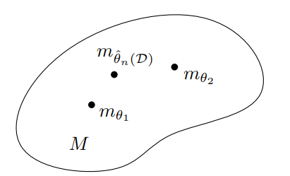
Parametrization of a Statistical Manifold (SM) is visualized by Fig. 1 [4].
According to the literature, a paper by [5] examined info-geometrically the stable M/D/1 queue based on queue length routes ‘characteristics, was the real motivator for the current study.
The main deliverables of this paper are described below.
I. The discovery of the FIM and its inverse for the transient M/M/ 1 queue.
II. Revealing the new discovery of the Geodesic Equations (GEs) of motion of the coordinates of the transient M/M/ 1 queue.
III. A novel -connection [6] is introduced, which maps each coordinate to a value.
IV. Highlighting potential IG applications to ML.
The remainder of the paper is divided into the following sections: preliminary IG definitions are given in Section 2. The transient M/M/1 QM’s FIM and it IFIM are introduced in Section 3. While Section 4 gives the Information Geometric Equations of Motion (IMEs) for the coordinates of the transient M/M/1 QM. Section V addresses IG applications to ML. Section VI wraps up the paper and provides some challenging open problems combined with further research.
1.1 Statistical Manifold
M = {p(x, θ)|θϵΘ} is called an SM [6] if x is a random variable in sample space X and p(x, θ) is the probability density function, which satisfies certain regular conditions.
2. Potential Function
The potential function Ψ(θ) [6] is the distinguished negative function of the coordinates alone of ℒ(x; θ) = l n(p(x; θ)).
3. Fisher’s Information Matrix
Fisher’s Information Matrix (FIM), namely [gij] reads as:
[g ] = [ (Ψ(θ))] , i, j = 1,2, . . , n. (1)
ij i j ∂θ ∂θ
With respect to natural coordinates.
4. Inverse Fisher Information Matrix (IFIM), Namely [ ]
ij
[g ] [6] reads:
adj[gij]
ij −1 (2)
[g ] = ([g ij]) ) = , ∆= det[gij].
5| -Connection
For each real number , the α- connection [7] reads:
(α) 1−α
Γ = ( )(∂i ∂j ∂k(Ψ(θ)). (3)
ij,k 2
With Ψ(θ) Definition (2), ∂i = .
∂θi
6. Geodesic Equations of Motion
The IEMs read as [6]
2 k i j
d θ k(0) dθ dθ k(α) (α) sk
+ Γ ( ) ( ) = 0,i, j = 1,2, … , n, Γ = Γ g . (4)
dt2 ij dt dt ij ij,s
By the above definition, the GEs are interpreted physically as the Information Geometric Equations of Motion , Shortly (IGEMs), or the Relativistic Equations of Motion (REMs) , or the Riemannian equations of motion. At this stage, the current study provides a ground- breaking discovery of the IG analysis of transient queueuing systems in comparison to that of non-time dependent queueing systems, namely IG analysis of stable queues [8], [9].
6.1 Fim And Ifim of the Transient M/M/1 Qm
The most straightforward probabilistic queueing model that can be studied analytically is a single-channel model with exponential inter-arrival durations, service times, and FIFO queue discipline. This is called the M/M/1 queue in queueing theory [10].
Based on the introduction of the function, Parthasarathy [10] suggested a straightforward method for the transient solution of the M/M/1 system to read as
−(λ+μ)t n (λ+μ)t
pn(t) = ρp0(t)e [∑m=1 rm (t) + e ], n = 0,1,2, …, (5)
where stands for the mean rate per unit time at which arrival instants occur, is the mean rate of service
λ(t)
time, ρ = defines the traffic intensity or utilization factor.
μ(t)
n−a1 n−1−a1
rn(t) = ( μβ (1 − δ0a )[In−a (β1t) − In+a (β1t)] + λβ (In+1−a (β1t) −
2 1 1 1 2 1
In−1−a (β1t))).
With β1 = 2√λμ , β2 = 2√ , In(x) Eq. (19) is the modified Bessel function and
−(λ+μ)y
p0(t) = ∫ r1 e dy + δ0a .
Theorem 1. The underlying queue of Eq. (5) has:
I. FIM reads as a b c
[gij] = [b 0 h]. (7)
c h l With
a = − , (8)
ρ2 (1−ρ)2
b = t, (9)
ρ ρ . .
c = + + tμ + μρ , (10)
ρ2 (1−ρ)2
h = (1 + ρ) + tρ , (11)
.2 .. .2 ..
ρ − ρρ ρ + (1 − ρ)ρ
.. . . . . .. (12)
l = ( + + ((1 + ρ)tμ + μ + 2ρ μ + 2μρ + 2ρμ + μtρ , 2 ( )2 ρ 1 − ρ
Δ = det([gij]) = (a(−h ) − b(bl − ch) + c(bh)). (13)
Provided that, . refers to the temporal derivative .
dt ij
II. [g ] reads as:
A B L
adj[gij] ij
[g ] = = [B E F], (14)
L F H where (−h )
A = , (15)
(ch − bl)
B = , (16)
(bh)
L = , (17)
(al − c )
E = , (18)
(bc − ah)
F = , (19)
(−b )
H = . (20)
III. Following (5), we have
−(λ+μ)t −(λ+μ)t n
ℒ(x; θ) = l n(pn(x; θ)) = (l n(ρp0(t)e ) + l n(ρp0(t)e [∑m=1 rm (t) +
(λ+μ)t (21)
e ] ),
θ = (θ1, θ2, θ3) = (ρ, μ, t). (22)
We have
Ψ(θ) = −l n(ρ) − l n(1 − ρ) + μ(1 + ρ)t, p0(t) = 1 − ρ. (23)
Thus,
∂Ψ 1 1 ∂Ψ ∂Ψ ρ ρ
∂1 = = − + + μt, ∂2 = = (1 + ρ)t , ∂3 = = − + + (1 +
∂ρ ρ (1−ρ) ∂μ ∂t ρ (1−ρ)
(24)
ρ)tμ + μ(1 + ρ) + μtρ ,
∂1 ∂1 = − , (25)
2 ( )2 ρ 1 − ρ
∂1 ∂2 = ∂2 ∂1 = t, (26) 2 2 = 0, (27)
ρ ρ . .
∂1 ∂3 = + + tμ + μρ = ∂3 ∂1,
ρ2 (1−ρ)2 (28)
∂2 ∂3 = (1 + ρ) + tρ = ∂3 ∂2, (29)
.2 .. .2 ..
ρ − ρρ ρ + (1 − ρ)ρ
.. . . . . ..
∂3 ∂3 = ( + + (1 + ρ)tμ + μ + 2ρ μ + 2μρ + 2ρμ μtρ ). (30)
2 ( )2 ρ 1 − ρ
Therefore, the fisher information matrix, FIM, is obtained (Eq. (7)).
ij
[g ] reads as:
a b c
adj[gij] Transpose(Cov[gij]) 1 ij −1
[g ] = [gij] = = = transpose(Cov [b 0 h])
∆ ∆ ∆
c h l
2 (31)
(−h ) (ch − bl) (bh) = [(ch − bl) (al − c ) (bc − ah)].
(bh) (bc − ah) (−b )
Thus,
(−h ) (ch − bl) (bh) A B L
ij 1 2
[g ] = transpose(Cov[(ch − bl) (al − c ) (bc − ah)]) = [B E F].
2 L F H (bh) (bc − ah) (−b )
As requested, It is notable that FIM should satisfy the symmetry requirement.
In what follows, the components of α (or ∇ )- connection are obtained. These calculated expressions are needed to obtain the corresponding GEs of the parametric coordinates of M/M/1 QM.
From Eq. (3), the reader can check that.
(α) 1 1
Γ = −(1 − α)( + ),
11,1 (1−ρ)3 ρ3 (32)
(α) (α) (α) (α) (α) (α) (α) (α) (α) (α)
0 = Γ22,2 = Γ12,2 = Γ22,1 = Γ21,2 = Γ11,2 = Γ12,1 = Γ21,1 = Γ22,3 = Γ = Γ32,2, (33)
23,2 (α) . 1 1
Γ = (1 − α)ρ ( − ),
31,1 (1−ρ)3 ρ3 (34)
(α) (α) 1 1
Γ = Γ = ( 1 − α)ρ ( − ), (35)
13,1 11,3 3 3
(1 − ρ) ρ
(α) (α) (1 − α)
Γ = Γ = , (36)
13,2 12,3 .. .. .2
( ) (1 − α) ρ ρ 2ρ
α .. .
Γ13,3 = [ + + + tμ + 2μ ], (37)
2 ( )2 ( )3 2 ρ 1 − ρ 1 − ρ
( ) ( ) (1 − α)ρ
Γ23,1 = Γ21,3 = , (38)
. ..
( ) (1 − α)(1 + 2ρ + tρ )
Γ23,3 = , (39)
( ) ( ) (1 − α) Γ31,2 = Γ32,1 = . (40) Engaging the same procedure, the remaining components can be determined.
6.2 The IGMES of the Underlying Queue Manifold
I. The IMEs of the server utilization coordinate, ρ of the transient M/M/1QM.
The IMEs corresponding to the arrival rate coordinate, ρ are
2 1 i j
d θ 1(0) dθ dθ
+ Γ ( ) ( ) = 0,i, j = 1,2,3.
dt2 ij dt dt
Now, we are in a situation of trying to find the path of motion of family of families of IMEs corresponding to the server utilization coordinate, ρ.
. 1 1
2Aρ ( − ) +
2 . (1−ρ)3 ρ3 d ρ L Lρ dρ dμ 1
[ + [ + ]( )( ) +[ ( .. .. .2 ) +
dt2 2 2 dt dt 2 ρ ρ 2ρ .. .
B + L [ + + + tμ + 2μ ]
ρ2 (1−ρ)2 (1−ρ)3
.. .2 .2 ..
1 . 1 1 ρρ −2ρ 2ρ +(1−ρ)ρ
(2Aρ ( − ) + B + ( + +
2 (1−ρ)3 ρ3 ρ3 (1−ρ)3 .. . . . .. dρ dt . 1 1 dρ 2
tμ + ρ μ + μ + μρ ) L))]( )( )+[ρ L( − )]( ) +
dt dt (1−ρ)3 ρ3 dt 1 . . .. 1 . .. dμ dt
[ (Aρ + B(1 + 2ρ + tρ )) + (A +(ρ + tρ )L)]( )( )+ (41)
2 2 dt dt
.. .2 .2 ..
1 ρρ −2ρ 2ρ +(1−ρ)ρ .. . . . .. .
[ (( + + tμ + ρ μ + μ + μρ ) A + (ρ +
2 ρ3 (1−ρ)3
. .. … . .2 .. . .. … . .2 ..
.. (ρ ρ −ρρ )ρ−2ρ (ρ −ρρ ) (ρ ρ +(1−ρ)ρ )(1−ρ)+2ρ (ρ +(1−ρ)ρ )
tρ )B +[ + +
ρ3 (1−ρ)3 ... .. . .. . .. . ..
(1 + ρ)tμ + (1 + ρ)μ + 3ρ μ + μ + 2ρ μ + 2μρ +
. . .. ... .. . .. dt
4μ ρ + 2ρμ + μtρ + μρ + μ tρ ]L)] ( ) ] = 0.
dt
It can be verified that one of the closed form solutions of Eq. (41) is determined by the paths of motion:
ρ(t) = constant, μ(t) = constant , such that ρ ∈ (0,1), μ > 1. (42)
II. The IMEs of the Mean service Rate coordinate, μ of the transient M/M/1 QM.
The IMEs of are
2 2 i j
d θ 1(0) dθ dθ
+ Γ ( ) ( ) = 0,i, j = 1,2,3.
dt2 ij dt dt
Now, we are in a situation of trying to find the path of motion of family of families of IMEs corresponding to the mean service rate, .
2 . .. .. .2
d μ F Fρ dρ dμ 1 . 1 1 ρ ρ 2ρ ..
[ + [ + ]( )( ) +[ (2Bρ ( − ) + E + F [ + + + tμ +
dt2 2 2 dt dt 2 (1−ρ)3 ρ3 ρ2 (1−ρ)2 (1−ρ)3
.. .2 .2 ..
. 1 . 1 1 ρρ −2ρ 2ρ +(1−ρ)ρ .. . . . ..
2μ ]) + (2Bρ ( − ) + E + ( + + tμ + ρ μ + μ + μρ )
2 (1−ρ)3 ρ3 ρ3 (1−ρ)3 dμ dt . 1 1 dρ 1 . . .. 1 .
F)]( ) ( )+[ρ ( − ) F] ( ) + [ (Bρ + E(1 + 2ρ + tρ )) + (B +(ρ +
dt dt (1−ρ)3 ρ3 dt 2 2
.. .2 .2 ..
.. dρ dt 1 ρρ −2ρ 2ρ +(1−ρ)ρ .. . . . .. .
tρ )F)]( )( )+[ (( + + tμ + ρ μ + μ + μρ ) B + (ρ +
dt dt 2 ρ3 (1−ρ)3
. .. … . .2 .. . .. … . .2 ..
.. (ρ ρ −ρρ )ρ−2ρ (ρ −ρρ ) (ρ ρ +(1−ρ)ρ )(1−ρ)+2ρ (ρ +(1−ρ)ρ )
tρ )E + [ + +
ρ3 (1−ρ)3
Thus, 1 1 .. . . 2
(( − )[ ((1+ρ)tμ +μ+2ρμ ]−(tμ ) )
ρ2 (1−ρ)2 1 1 2
(( − )(−((1+ρ)) )−(t2[((1+ρ)tμ..+μ+2ρμ.]))
2 ρ2 (1−ρ)2
d μ 1
[ +[ 1 1 +
dt2 2 .
(t(tμ )−( − )(1+ρ))
ρ2 (1−ρ)2
.. .
[tμ + 2μ ]
1 1 2 2 .. .
(( − )(−((1+ρ)) )−(t [((1+ρ)tμ +μ+2ρμ ]))
ρ2 (1−ρ)2
. 1 1
(t(tμ )−( − )(1+ρ))
ρ2 (1−ρ)2
+ (43)
1 1 2
(( − )(−((1+ρ)) )−(t2[((1+ρ)tμ..+μ+2ρμ.]))
ρ2 (1−ρ)2
. 1 1
(t(tμ )−( − )(1+ρ))
ρ2 (1−ρ)2
.. . dμ 1 ..
(tμ + μ ) )]( )+[ (( tμ +
1 1 2 dt 2 (( − )(−((1+ρ)) )−(t2[((1+ρ)tμ..+μ+2ρμ.]))
ρ2 (1−ρ)2 . ..
. (tμ (1−ρ)−t[((1+ρ)tμ +μ])
μ ) +] ] = 0.
1 1 2
(( − )(−((1+ρ)) )−(t2[((1+ρ)tμ..+μ+2ρμ.]))
ρ2 (1−ρ)2
It is obvious that for arbitrary constant values of ρ, μ, we have a closed form solution for Eq. (43). As time becomes sufficiently large, i.e., t → ∞, Eq. (42) reduces to
.. .2 . ...
3μ 3μ μ μ
[ − − ] = 0. (44)
2 2(1+ρ) μ..
2γt
We propose the closed form solution, μ = , for some arbitrary non-zero constant . substituting in Eq.
(1+γt)
(44) implies:
18γ + + 6γ = 0. (45) (1 + γt)(1 + ρ)
As t → ∞, γ = 0,0,0, −3. The only accepted value is γ = −3, μ = , which tends to the value μ = 2 as
(3t−1)
t → ∞.
III. The IMEs of the temporal coordinate, t for the underlying QM.
Engaging a similar lengthy mathematical manipulation, it can be verified that the IMEs of the temporal coordinate, t, at infinite time is characterized by the family of families of temporal curves:
μ(t) = ζ1+ζ2t + ζ3t . (46)
for some arbitrary non-zero constants ζ1,ζ2, ζ3, 1 > 1.
IV. Ig Applications To Ml Stochastic gradient descent is a popular optimisation approach in ML that seeks to determine which direction of descent is the steepest within probability distributions’ parameter space. Amari et al. [11] created the natural gradient, which is superior to the ordinary gradient since it more accurately captures this direction. Furthermore, even with gradient descent, FIM can be used to calculate the predicted change in output about parameter changes. Artificial Neural Networks (ANNs) are functions with multiple parameters that map input vectors to output vectors. They are widely applied in regression, computer vision, and speech processing. ANNs can be trained through supervised learning, where a training set of input-output pairs is used, or through unsupervised learning, which does not require a training set. The back-propagation algorithm efficiently computes the gradient descent by determining the contribution of each parameter to the error. Overfitting, a common issue in ANNs, can be mitigated by techniques such as using a validation set, early stopping, data augmentation, and dropout [12].
In Reinforcement Learning (RL) [13], when an agent needs to prepare for unknown tasks, one approach is unsupervised skill discovery. These algorithms learn a set of policies without using a reward function and are like representation learning algorithms in supervised learning. While prior work has shown that these methods can accelerate downstream tasks, our analysis reveals that they do not learn skills that are optimal for every possible reward function. However, the distribution over skills can provide an optimal initialization that minimizes regret against adversarially chosen reward functions, assuming a specific adaptation procedure. Notably, understanding which state marginals are achievable is crucial for analyzing the behavior of unsupervised skill learning algorithms [13] and their relevance to state-dependent reward functions. The set of achievable state marginal distributions can be characterized by a set of linear equations or by a complementary description based on a specific property.
This alternative perspective provides insights into the relationship between learned skills and downstream tasks in RL. So, if we have a set of possible state distributions, any combination of those distributions within the convex hull is also possible. This means that there exists a policy that can achieve any state distribution within that convex hull. By taking the convex hull of the state distributions of all deterministic policies, we can obtain the set of all possible state distributions, which is referred to as a polytope. Each vertex of the polytope represents a deterministic policy, and any policy's state distribution can be expressed as a combination of the state distributions at the vertices, as visualized by Fig. 2.
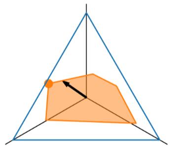
The objective of maximizing the expected return is equivalent to maximizing the dot product between the state marginal distribution and the reward vector. This visualization helps us understand how different reward-maximizing policies are related to the state marginal polytope and provides insights into the relationship between state-dependent reward functions and optimal policies [13].
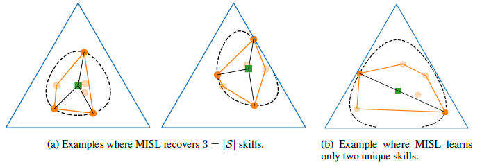
The analysis of where the skills learned by Mutual Information-based Skill Learning (MISL) are positioned on the state marginal polytope, which has motivated [13] to undertake this analysis by examining the mutual information objective and dissecting it to understand how the learned skills align with the polytope. In the context of skill learning [13], maximizing mutual information is equivalent to minimizing the maximum difference between a prior distribution over states (represented by a green square) and any possible state distribution.
This concept, known as information geometry, helps optimize skill-learning algorithms by assigning higher probabilities to policies with state distributions that deviate further from the average state distribution. The goal is to find skills as distinct as possible from each other and the average state distribution. Most importantly, the opaque circles represent the skills discovered by the Mutual Information Skill Learning (MISL) algorithm. The dashed line represents equidistant state marginals from the green square, indicating an equal divergence from the prior distribution over states. This visualization helps illustrate the relationship between the skills learned by MISL and their distribution in relation to the average state distribution. This is illustrated in Fig. 3. Reliable detection of Out-Of-Distribution (OOD) samples [14] is crucial for ensuring the safety of modern machine learning systems. The work of [14] introduced IGEOOD, an effective method that can detect OOD samples using any pre-trained neural network, regardless of the level of access to the ML model. By leveraging the geodesic distance between data distributions, IGEOOD combines confidence scores from the neural network's logits outputs and learned features to achieve superior performance compared to other state-of-the-art methods across different network architectures and datasets [14].
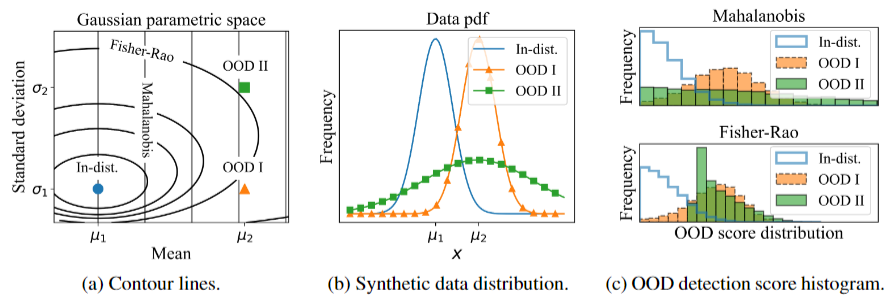
The authors [14] introduced the concept of IG and derived a metric based on the Fisher-Rao distance to measure the mismatch between probability density functions of a pre-trained neural classifier. Experimental results demonstrate that IGEOOD performs competitively with state-of-the-art methods in different setups, including black-box and grey-box scenarios, and achieves improved performance on various benchmarks. Fig. 4 showcases a comparison between Fisher-Rao and Mahalanobis distances for distinguishing between 1D Gaussian distributions in the context of OOD detection. It highlights the motivation to use the Fisher-Rao metric, which measures the dissimilarity between probability models, as it shows better performance in distinguishing between in-distribution and OOD samples compared to other distance-based approaches.
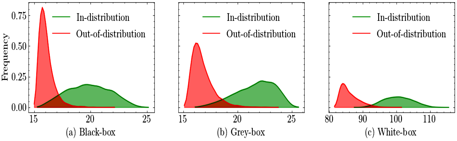
In the context of the experiment, the authors [14] compared three different settings for OOD detection. They use a unified metric, but with different formulations based on the type of distribution. For the Deep Neural Network (DNN) outputs, they use the softmax posterior probability distribution, while for the intermediate layers, they employ a model based on diagonal Gaussian Probability Density Functions (PDFs). This unified framework combines a single distance measure for both the softmax outputs and the latent features of the neural network, contributing to the separation of in-distribution and OOD samples, as illustrated in Fig. 5. The distributions are shown for three different settings, specifically for a pre-trained DenseNet model on CIFAR-10 dataset, considering both in-distribution and OOD data from TinyImageNet (downsampled). This analysis helps evaluate the effectiveness of the IGEOOD score in distinguishing between in-distribution and OOD samples [13].
7. Conclusion
This study offers a revolutionary info-geometrics of transient M/M/1 QM. For this queue, FIM and IFIM are established. The GEs of motion for the queue's coordinates are determined. More potentially, some IG applications to ML are provided. Here are some challenging open problems to be addressed.
Open problem one: following the analysis in [13], a simplified model of skill learning algorithms that treated policy parameters and latent codes as a single representation, with different skills having distinct parameter sets was employed. However, practical implementations of skill learning algorithms are less flexible, which can alter the shape of the state marginal polytope.
This limited flexibility may lead to incomplete representation of certain state distributions, resulting in gaps or divisions in the polytope. It is yet to be determined if these practical implementations learn fewer unique skills and how these limitations impact the average state distribution, which is a really challenging open problem.
Open problem two: following the derivation of the potential function, PF.
Ψ(θ) = −l n(ρ) − l n(1 − ρ) + μ(1 + ρ)t, p0(t) = 1 − ρ.
Is the process of finding the threshold of PF based on its parameters decidable? The problem is still open. Open problem three: having discovered PF (Eq. (21)), is it feasible to examine its algebraic properties as well as doing the same for its inverse, if it exists? This is a challenging open problem, yet unsolved so far.
Open problem four: the discovery of Revolutionary relativistic connections with the investigated transient queue is still unsolvable problem, for example finding the corresponding Gaussian,Ricci, Scalar and Einesteinian tensors for the transient M/M/1 QM.
The frontiers are open for unlimited explorations. The next phase of research includes answering the above open research problems and exploring more new avenues of IG applications to other scientific disciplines. More importantly, the possibility of employing Riemannian Geometric (RG) analysis, and the Theory of Relativity (TR) to the analysis of the dynamics of transient queues.
Conflict of Interest
The authors declare no conflict of interest.
Data Availability
All data are included in the text.
Funding
This research received no specific grant from funding agencies in the public, commercial, or not-for-profit sectors.
References
- [1] Mageed, I. A., Zhou, Y., Liu, Y., & Zhang, Q. (2023). Towards a revolutionary info-geometric control theory with potential applications of fokker planck kolmogorov (fpk) equation to system control, modelling and simulation [presentation]. 2023 28th international conference on automation and computing (icac) (pp. 1–6). https://doi.org/10.1109/ICAC57885.2023.10275271
- [2] Skoda, Z. (2019). Information geometry. https://ncatlab.org/nlab/show/information+geometry
- [3] Mageed, I. A., Zhang, Q., Akinci, T. C., Yilmaz, M., & Sidhu, M. S. (2022). Towards abel prize: the generalized brownian motion manifold’s fisher information matrix with info-geometric applications to energy works. 2022 global energy conference (GEC) (pp. 379–384). IEEE. DOI: 10.1109/GEC55014.2022.9987239
- [4] Mageed, I. A., Yin, X., Liu, Y., & Zhang, Q. (2023). Za,b of the stable five-dimensional M/G/1 queue manifold formalism’s info- geometric structure with potential info-geometric applications to human computer collaborations and digital twins. 28th international conference on automation and computing (ICAC) (pp. 1–6). IEEE. DOI: 10.1109/ICAC57885.2023.10275185
- [5] Nakagawa, K. (2002). The geometry of M/D/1 queues and Large Deviation. International transactions in operational research, 9(2), 213–222.
- [6] Peng, L., Sun, H., & Jiu, L. (2007). The geometric structure of the Pareto distribution. Boletin de la asociación matemática venezolana, 14(1–2), 5–13.
- [7] Dodson, C. T. J. (2005). Topics in information geometry. The University of Manchester.
- [8] Mageed, I. A., & Kouvatsos, D. D. (2019). Information geometric structure of stable M/G/1 queue manifold and its matrix exponential. 35th uk performance engineering workshop 16 december 2019 (p. 116). IEEE. https://www.researchgate.net/profile/Dr-Vijay-Singh-2/publication/340951179_proceedings/links/5ea70fb145851553fab34b07/proceedings.pdf#page=123
- [9] Mageed, I. A., & Kouvatsos, D. D. (2021). The impact of information geometry on the analysis of the stable M/G/1 queue manifold. ICORES (pp. 153–160). DOI: 10.5220/0010206801530160
- [10] Parthasarathy, P. R. (1987). A transient solution to an M/M/1 queue: a simple approach. Advances in applied probability, 19(4), 997–998.
- [11] Amari, S., Ozeki, T., Karakida, R., Yoshida, Y., & Okada, M. (2017). Dynamics of learning in MLP: Natural gradient and singularity revisited. Neural computation, 30(1), 1–33. https://bsi-ni.brain.riken.jp/database/file/349/349.pdf
- [12] Mageed, I. A., & Zhang, K. Q. (2022). Information geometry? exercises de styles. Electronic journal of computer science and information technology, 8(1), 9–14.
- [13] Eysenbach, B., Salakhutdinov, R., & Levine, S. (2021). The information geometry of unsupervised reinforcement learning. https://arxiv.org/abs/2110.02719
- [14] Gomes, E. D. C., Alberge, F., Duhamel, P., & Piantanida, P. (2022). Igeood: an information geometry approach to out-of-distribution detection. https://arxiv.org/abs/2203.07798