
Solving Vendor Selection Problem by Interval Approximation of Piecewise Quadratic Fuzzy
Abstract
In this paper, a Vendor Selection Problem (VSP) with fuzzy parameter uncertainty is introduced. The buyer gives a quantity order for a commodity among a set of suppliers. Buyer’s objective is to obtain the requirements of lead time, service level and aggregate quality at the minimum cost. Some of the problem parameters are characterized by the piecewise quadratic fuzzy numbers. In addition, an interval approximation for piecewise quadratic fuzzy numbers is proposed for solving the VSP. The VSP with close interval approximation is approached by taking the minimum and maximum values inequalities with the constraints transformed it to two classical Linear Programming Problems (LPPs). The optimal solution for these LPPs is obtained. A numerical example is provided for illustration of the suggested approach.
Keywords:Close interval approximationFuzzy optimal solutionPiecewise quadratic fuzzy numbersVendor
selection.
1. Introduction
In the literature, Vendor Selection Problem (VSP) was studied by Dickson [1]. First, Zadeh [2] proposed the philosophy of fuzzy sets. Fuzzy decision-making was developed by Zimmermann [3], where they introduced fuzzy programming and LPP with multiple objective functions. Later, several researchers worked on various applications based on fuzzy uncertainty. Dubois and Prade [4] investigated the theory and applications of fuzzy uncertainty. Kaufmann and Gupta [5] studied several fuzzy mathematical models with their applications to engineering and management sciences. Maleki et al. [6] proposed a very effective method to solve a LPP including the fuzzy variables and the comparison of fuzzy numbers.
Many authors [7]–[9], studied the problems where all the parameters are uncertain. Lai and Hwang [10] assumed that the parameters might be characterized by triangular possibility distribution; then, they proposed an auxiliary model, which was solved by applying the multi-objective LPP.
Weber and Current [11] studied the multiple objective methods for solving the VSP. Several authors used fuzzy multi-objective approaches to VSP, like [12]–[15], studied the manufacturing delivery performance problem with an application to supply chain management, further investigated by Carvalho and Costa [16]. Several researchers studied the modified S-curve membership function in VSP, for example, Vasant, M. [17], Madroñero [18], Torabi and Hassini [19] presented a novel method based on possibilistic programming to solve a multi-objective supply chain model. Selim and Ozkarahan [20] addressed a supply chain model integrated with network design, which an interactive fuzzy goal programming method solved. Many papers integrated fuzzy and stochastic uncertainty with VSP to determine the performance of suppliers and choose the suitable supplier are those of [21]–[24], and many more. Several papers have been published in green supplier selection in the last few decades. For instance, Jain et al. [25] studied a buyer-initiated decision-making process with the inclusion of the green supplier selection concept.
Luthra et al. [22] investigated a method to solve the sustainable VSP further extended by Chen and Zou [26]. Ehsan et al. [10] studied the green VSP using a MODM algorithm. Ghaniabadi and Mazinani [27] presented a dynamic lot size model for multiple suppliers. Turk et al. [28] studied the multi-objective model in inventory management with supplier selection. Aouadni et al. [29] presented a detailed survey on VSP as well as order allocation problems. This study investigates the approximation of close interval for piecewise quadratic fuzzy to solve the VSP. The remaining portion of the work is arranged as follows. Section 2 recalls some basic concepts needed. Section 3 introduces VSP as an LPP. Section 4 formulates the piecewise quadratic fuzzy VSP. Section 5 provides a numerical example to support and validate the proposed methodology. In the end, a few concluding remarks are reported in Section 6.
2. Basic Concepts
In this section, some basic terms and results are recalled.
Definition 1 ([30]). A piecewise quadratic fuzzy number (PQFN) is denoted by a ̃PQ = (a1, a2, a3, a4, a5), where a1 ≤ a2 ≤ a3 ≤ a4 ≤ a5 are reals, is defined by its membership function a ̃ as follows (Fig. 1).
PQ
0, x < a1, (x − a1) , a1 ≤ x ≤ a2, ( )2 2 a2 − a1 (x − a3) + 1, a2 ≤ x ≤ a3, ( )2 2 a3 − a2
μa ̃ = 1 1 (1)
PQ 2
(x − a3) + 1, a3 ≤ x ≤ a4, ( )2 2 a4 − a3 (x − a5) , a4 ≤ x ≤ a5, ( )2 2 a5 − a4 0, x > a5.
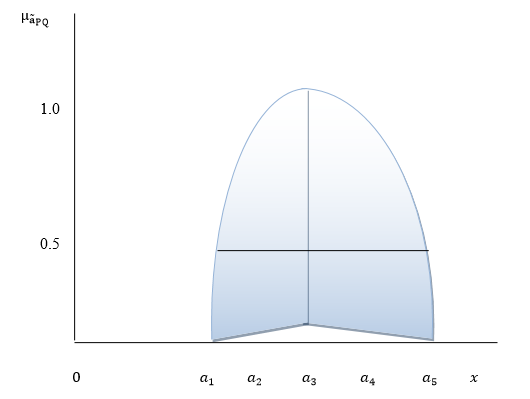
The interval of confidence at level α for the PQFN is defined as (a ̃PQ) = Lα(a ̃PQ) = [a1 + 2(a2 − a1)α, a5 − 2(a5 − a4)α] for all α ∈ [0,1].
L U ̃
Definition 2 ([30]). An interval approximation [A] = [aα, aα] of a PQFN A is referred to as a closed interval approximation if aα = inf{x ∈ ℜ: μ̃ ≥ 0.5}, and aα = sup{x ∈ ℜ: μ̃ ≥ 0.5}.
Definition 3 ([30]). The associated ordinary numbers of PQFN corresponding to [A] = [aα, aα ] is [A] =
L U aα+aα
[a , a ] is equal to A ̂ = .
Definition 4 ([30]). Suppose that a ̃ = (a , a , a , a , a ) and b ̃ = (b , b , b , b , b ) be two PQFNs. Then
PQ 1 2 3 4 5 PQ 1 2 3 4 5
I. Addition: a ̃ ⊕ b ̃ = (a + b , a + a , a + b , a + b , a + b ).
PQ PQ 1 1 2 2 3 3 4 4 5 5
II. Scalar multiplication: α. a ̃PQ = (α a1, α a2, α a3, α a4, α αa5), α > 0.
L U L U
Definition 5 ([30]). Let [A] = [(aα) , (aα) ], and [B] = [(bα) , (bα) ] be two interval approximations of PQFN. Then, two define the arithmetic operations as follows:
L L U U
I. Addition: [A] ⊕ [B] = [A] ⊕ [B] = [aα + bα, aα + bα].
L U U L
II. Subtraction: [A] ⊖ [B] = [aα − bα, aα − bα].
[α aα, α aα], α > 0,
III. Scalar multiplication: α [A] = {
[α aα, α aα], α < 0.
U L L U L L U U
aαbα+aαbα aαbα+aαbα
IV. Multiplication: [A] ⊙ [B] = [ , ].
2aα 2aα L U
[ , ] , [B] > 0 and bα + bα ≠ 0,
L U L U
[A] bα+ bα bα+ bα
V. Division: = {
[ ] U L B 2aα 2aα
[ , ] , [B] < 0 and bα + bα ≠ 0.
L U L U
bα+ bα bα+ bα
VI. The order relations (≈, ≅, ≲, ≳) are defined as
L L U U
I. Fuzzy equal: [A] ≈ [B] if aα = bα and aα = bα.
L U L U
II. Fuzzy equivalent: [A] ≅ [B] if aα + aα = bα + bα.
L L U U L U L U
III. [A] ≲ [B] if aα ≤ bα and aα ≤ bα , or aα + aα ≤ bα + bα .
L U U L
IV. [A] ≳ [B] if aα ≥ bα and aα ≥ bα.
3. Vendor Selection Problem
A VSP is defined as a LPP for minimizing price under the restriction of quality performance measures, services, and lead time is provided as [21]
min ( ) = ∑ pixi.
∑ qixi ≥ Q,
∑ sixi ≥ S,
∑ lixi ≤ L,
∑ xi = 1,
xi ≥ 0 for all .
Where xi: fraction of demand allocated to vendor i.
pi: price of item i.
qi: quality level of item i.
li: lead time of item i.
si: level of service of item i.
Q: required overall quality level.
L: lead time level.
S: service level.
4. Piecewise Quadratic Fuzzy VSP
Consider the following PQFVS using the close interval approximation as min ( ) = ∑ [pi]xi.
∑ [qi]xi ≥ [Q],
∑ [si]xi ≥ [S] ,
∑ [li]xi ≤ [L],
∑ xi = 1,
xi ≥ 0 for all .
Where [li] = [(li)α, (li)α ], [pi] = [(pi)α, (pi)α], [qi] = [(qi)α, (qi)α], [si] = [(si)α, (si)α ], [L] = [Lα, Lα], [Q] = [Qα, Qα], [S] = [Sα, Sα ] ∈ P(ℜ).
P(ℜ )=set of all close interval approximations on ℜ.
Definition 6. Any xj which satisfies the constraints in Problem (2) is referred to as a feasible solution. Let G be the set of all feasible solutions of Problem (1). We claim that x ∈ G is said to be an optimal solution only when [p]x ≤ [p]x for all x ∈ G.
Lemma 1. Problems (1) and (2) are equivalent.
Proof: let G1 and G2 denote the respective two feasible solution sets of Problems (1) and (2). Then, an element x ∈ G1 if and only if
∑ [qi]xi ≥ [Q],
∑ [si]xi ≥ [S],
∑ [li]xi ≤ [L],
∑ xi = 1.
If and only if
L U L U
∑ [(qi)α, (qi)α]xi ≥ [Qα, Qα],
L U L U
∑ [(si)α, (si)α]xi ≥ [Sα, Sα ],
L U L U
∑ [(li)α, (li)α]xi ≤ [Lα, Lα],
∑ xi = 1.
If and only if
L U L U
∑ [(qi)αxI, (qi)αxi] ≥ [Qα, Qα],
L U L U
∑ [(si)αxi, (si)αxi] ≥ [Sα, Sα ],
L U L U
∑ [(li)αxI, (li)αxi] ≤ [Lα, Lα],
∑ xi = 1.
If and only if m L U L U
(qi)α + (qi)α Qα + Qα ∑ ( )xi ≥ ( ), I=1 2 2
m L U L U
(si)α + (si)α Sα + Sα ∑ ( ) xi ≥ ( ), i=1 2 2
m L U L U
(li)α + (li)α Lα + Lα ∑ ( ) xi ≤ ( ), I=1 2 2 ∑ xi = 1.
If and only if
∑ qixi ≥ Q ,
∑ sixi ≥ S,
∑ lixi ≤ L,
∑ xi = 1.
If and only if x ∈ G2.
Hence G1 ≅ G2.
Let X be the optimal feasible solution of Problem (2), then we obtain.
[P]X ≤ [P]X for all X ∈ G1.
If and only if ∑ [pi]xi ≤ ∑ [pi]xi for all xj ∈ G1,
i=1 i=1
If and only if
m L U m L U
(pi)α + (pi)α (pi)α + (pi)α ∑ ( ) xi ≤ ∑ ( ) xi, i=1 2 i=1 2 If and only if ∑ pixi ≤ ∑ pixi .
i=1 i=1
Thus, we have X is an optimal feasible solution of the crisp VSP as given by (1).
Referring to the interval arithmetic operations [31] Problem (2) is converted into 2 inequalities as follows:
L U U L
∑ (qi)αxi ≥ Qα , ∑ (qi)αxi ≥ Qα ,
i=1 i=1 L U U L
∑ (si)αxi ≥ Sα , ∑ (si)αxi ≥ Sα,
i=1 i=1 L L U U
∑ (li)αxi ≤ Lα , ∑ (li)αxi ≤ Lα,
i=1 i=1
∑ xi = 1,
xi ≥ 0 for all .
Let Gi be a set of solutions to the i inequality and define.
2m+1 2m+1
G = ⋃i=1 Gi and G = ⋂i=1 Gi.
m (i) (i) m (i) (i) m (i) (i)
Definition 7. Suppose that: ∑i=1[q , q ]xi ≥ [Q1, Q2], ∑i=1[s , s ]xi ≥ [S1, S2] and ∑i=1[l , l ]xi ≥
1 2 1 2 1 2 m (i) m (i) m (i)
[L1, L2]. Then inequalities ∑i=1 q xi ≥ Q, ∑i=1 s xi ≥ S and ∑i=1 l xi ≥ L are called the characteristic
m (i) (i) m (i) (i) m (i) (i)
formulas of ∑i=1[q , q ]xi ≥ [Q1, Q2], ∑i=1[s , s ]xi ≥ [S1, S2] and ∑i=1[l , l ] ≥ [L1, L2]; respectively.
1 2 1 2 1 2 (i) (i) (i) (i) (i) (i) (i) (i) (i)
Here, q ∈ [q , q ], s ∈ [s , s ], and l ∈ [l , l ].
1 2 1 2 1 2 m (i) (i) m (i) (i)
Definition 8. For each inequality ∑i=1[q , q ]xi ≥ [Q1, Q2], ∑i=1[s , s ]xi ≥
1 2 1 2 m (i) (i)
[S1, S2] and ∑i=1[l , l ]xi ≥ [L1, L2] if there is one characteristic formula such that its solution set is similar to G or G, in this case, we say that the characteristic formulas as maximum and minimum values range inequalities.
m (i) (i) m (i) (i)
Proposition 1. Let the following inequalities ∑i=1[q , q ]xi ≥ [Q1, Q2], ∑i=1[s , s ]xi ≥
1 2 1 2 m (i) (i) m L U m U
[S1, S2] and ∑i=1[l , l ]xi ≥ [L1, L2]. Then, we have ∑i=1(qi)αxi ≥ Qα, ∑i=1(qi)αxi ≥
L m L U m U L m L L m U U
Qα , ∑i=1(si)αxi ≥ Sα , ∑i=1(si)αxi ≥ Sα, ∑i=1(li)αxi ≤ Lα , ∑i=1(li)αxi ≤ Lα are maximum and minimum values range inequalities for these constraint conditions, respectively.
By the arithmetic operations of intervals, Problem (2) is reduced into the following problems as
min ( ) = ∑ (pi)α xi.
∑ (qi)αxi ≥ Qα,
∑ (qi)αxi ≥ Sα ,
∑ (li)αxi ≤ Lα,
∑ xi = 1,
xi ≥ 0 for all i.
Now, we obtain the following optimization problem:
min ( ) = ∑ (pi)α xi.
∑ (qi)αxi ≥ Qα,
∑ (qi)αxi ≥ Sα ,
∑ (qi)αxi ≥ Sα ,
∑ (li)αxi ≤ Lα,
∑ xi = 1,
xi ≥ 0 for all i.
Suppose that the optimal solutions to Problems (3) and (4) are
∗ ∗ ∗ ∗ ∗∗ ∗∗ ∗∗ ∗∗
x1, x2, … , xm; Z1, x1 , x2 , … , xm; Z2 .
Thus, the optimal solution to the close interval approximation Problem (2) is ∗ ∗∗
minZ(x) = [Z1, Z2 ].
∗ ∗∗
x1 [x , x ] x ∗ ∗∗ 2 [x2, x1 ]
= . (5)
[x ] ∗ ∗∗ m [[xm, xm ]]
5. Numerical Example
Consider the following piecewise quadratic fuzzy VSP as in Table 1.
Table 1. Vendor's source piecewise quadratic fuzzy data.
This table is shown in the PDF version of the article.
The close interval approximations for the problem are presented in Table 2.
Table 2. Vendor's source close interval approximation data.
This table is shown in the PDF version of the article.
Applying Problem (2) to these data minZ(x) = [9, 11]x1 ⊕ [10, 11.5]x2 ⊕ [10.5, 12]x3.
[0.80, 0.95]x1 ⊕ [0.87, 0.97]x2 ⊕ [0.92, 1.02]x3 ≥ [0.80, 0.85], [0.80, 0.95]x1 ⊕ [0.92, 1.00]x2 ⊕ [0.90, 1.00]x3 ≥ [0.75, 0.80], [20, 35]x1 ⊕ [20, 30]x2 ⊕ [25, 27] 3 ≤ [20, 30], x1 + x2 + x3 = 1.0, x1, x2, x3 ≥ 0.
The interval Problem (6) is reduced to the following two LPPs as follows:
minZ1(x) = 9x1 + 10x2 + 10.5x3.
0.95x1 + 0.97x2 + 1.02x3 ≥ 0.80, 0.95x1 + 1.00x2 + 1.00x3 ≥ 0.75, 35x1 + 30x2 + 27 3 ≤ 30, x1 + x2 + x3 = 1.0, x1, x2, x3 ≥ 0.
Equivalently, we have the following problem.
minZ2(x) = 11x1 + 11.5x2 + 12x3.
0.80x1 + 0.87x2 + 0.92x3 ≥ 0.85, 0.80x1 + 0.92x2 + 0.90x3 ≥ 0.80, 20x1 + 20x2 + 25 3 ≤ 20, x1 + x2 + x3 = 1.0, x1, x2, x3 ≥ 0.
The solutions to the two Problems (7) and (8) are given below:
∗ ∗∗
1 [x1, x1 ] [0.2857, 0.375]
∗ ∗∗ ∗ ∗∗
[ 2] = [[x2, x2 ]] = [ [0, 0.7143] ] and minZ(x) = [Z1, Z2 ] = [9.9375, 11.3517].
∗ ∗∗
3 [x3, x3 ] [0, 0.625]
6. Conclusions
The VSP as an application of fully fuzzy LPP has been studied. The VSP with close interval approximation has been approached by taking the minimum and maximum value inequalities with the constraints reduced into two classical LPPs. The presented model possesses great future scope for development. One may consider the time value coefficients for more realistic objective function calculations. In addition, the model can be extended in the form of a multi-stage stochastic programming approach. As another future research direction, one may consider some more efficient algorithms to demonstrate the suggested model.
Conflicts of Interest
The authors declare no conflicts of interest to report regarding the present study.
References
- [1] Dickson, G. W. (1966). An analysis of vendor selection systems and decisions. Journal of purchasing, 2(1), 5–17. https://onlinelibrary.wiley.com/doi/abs/10.1111/j.1745-493X.1966.tb00818.x
- [2] Zadeh, L. A. (1965). Fuzzy sets. Information and control, 8(3), 338–353. https://www.sciencedirect.com/science/article/pii/S001999586590241X
- [3] Zimmermann, H. J. (1978). Fuzzy programming and linear programming with several objective functions. Fuzzy sets and systems, 1(1), 45–55. https://www.sciencedirect.com/science/article/pii/0165011478900313
- [4] Dubois, D. J. (1980). Fuzzy sets and systems: theory and applications. Elsevier science. https://books.google.com/books?id=JmjfHUUtMkMC
- [5] Kaufmann, A., & Gupta, M. M. (1988). Fuzzy mathematical models in engineering and management science. Elsevier science. https://dl.acm.org/doi/abs/10.5555/576010
- [6] Maleki, H. R., Tata, M., & Mashinchi, M. (2000). Linear programming with fuzzy variables. Fuzzy sets and systems, 109(1), 21–33. https://www.sciencedirect.com/science/article/pii/S0165011498000669
- [7] Buckley, J. J. (1988). Possibilistic linear programming with triangular fuzzy numbers. Fuzzy sets and systems, 26(1), 135–138. https://www.sciencedirect.com/science/article/pii/0165011488900139
- [8] Buckley, J. J. (1989). Solving possibilistic linear programming problems. Fuzzy sets and systems, 31(3), 329–341. https://www.sciencedirect.com/science/article/pii/0165011489902042
- [9] Lai, Y. J., & Hwang, C. L. (1992). A new approach to some possibilistic linear programming problems. Fuzzy sets and systems, 49(2), 121–133. https://www.sciencedirect.com/science/article/pii/016501149290318X
- [10] Lai, Y. J., & Hwang, C. L. (1992). Fuzzy mathematical programming. In Fuzzy mathematical programming: methods and applications (pp. 74–186). Berlin, Heidelberg: Springer Berlin Heidelberg. https://doi.org/10.1007/978-3-642-48753-8_3
- [11] Weber, C. A., & Current, J. R. (1993). A multiobjective approach to vendor selection. European journal of operational research, 68(2), 173–184. https://www.sciencedirect.com/science/article/pii/0377221793903013
- [12] Amid, A., Ghodsypour, S. H., & O’Brien, C. (2006). Fuzzy multiobjective linear model for supplier selection in a supply chain. International journal of production economics, 104(2), 394–407. https://www.sciencedirect.com/science/article/pii/S0925527305001532
- [13] Kumar, M., Vrat, P., & Shankar, R. (2006). A fuzzy programming approach for vendor selection problem in a supply chain. International journal of production economics, 101(2), 273–285. https://www.sciencedirect.com/science/article/pii/S0925527305000423
- [14] Mukherjee, S., & Kar, S. (2013). A three phase supplier selection method based on fuzzy preference degree. Journal of king saud university-computer and information sciences, 25(2), 173–185. https://www.sciencedirect.com/science/article/pii/S1319157812000419
- [15] Choi, J., Bai, S. X., Geunes, J., & Edwin Romeijn, H. (2007). Manufacturing delivery performance for supply chain management. Mathematical and computer modelling, 45(1), 11–20. https://www.sciencedirect.com/science/article/pii/S0895717705005327
- [16] de Carvalho, R. A., & Costa, H. G. (2007). Application of an integrated decision support process for supplier selection. Enterprise information systems, 1(2), 197–216. https://doi.org/10.1080/17517570701356208
- [17] Vasant, P. M. (2005). Solving fuzzy linear programming problems with modified s-curve membership function. International journal of uncertainty, fuzziness and knowledge-based systems, 13(01), 97–109. https://doi.org/10.1142/S0218488505003321
- [18] Díaz-Madroñero, M., Peidro, D., & Vasant, P. (2010). Vendor selection problem by using an interactive fuzzy multi-objective approach with modified S-curve membership functions. Computers & mathematics with applications, 60(4), 1038–1048. https://www.sciencedirect.com/science/article/pii/S0898122110002506
- [19] Torabi, S. A., & Hassini, E. (2008). An interactive possibilistic programming approach for multiple objective supply chain master planning. Fuzzy sets and systems, 159(2), 193–214. https://www.sciencedirect.com/science/article/pii/S0165011407003739
- [20] Selim, H., & Ozkarahan, I. (2008). A supply chain distribution network design model: an interactive fuzzy goal programming-based solution approach. The international journal of advanced manufacturing technology, 36(3), 401–418. https://doi.org/10.1007/s00170-006-0842-6
- [21] He, S., Chaudhry, S. S., Lei, Z., & Baohua, W. (2009). Stochastic vendor selection problem: chance-constrained model and genetic algorithms. Annals of operations research, 168(1), 169–179. https://doi.org/10.1007/s10479-008-0367-5
- [22] Luthra, S., Govindan, K., Kannan, D., Mangla, S. K., & Garg, C. P. (2017). An integrated framework for sustainable supplier selection and evaluation in supply chains. Journal of cleaner production, 140, 1686–1698. https://www.sciencedirect.com/science/article/pii/S0959652616314196
- [23] Ishibuchi, H., & Tanaka, H. (1990). Multiobjective programming in optimization of the interval objective function. European journal of operational research, 48(2), 219–225. https://www.sciencedirect.com/science/article/pii/037722179090375L
- [24] Karsak, E. E., & Dursun, M. (2015). An integrated fuzzy MCDM approach for supplier evaluation and selection. Computers & industrial engineering, 82, 82–93. https://www.sciencedirect.com/science/article/pii/S0360835215000388
- [25] Jain, V., Kumar, S., Kumar, A., & Chandra, C. (2016). An integrated buyer initiated decision-making process for green supplier selection. Journal of manufacturing systems, 41, 256–265. https://www.sciencedirect.com/science/article/pii/S0278612516300619
- [26] Chen, W., & Zou, Y. (2017). An integrated method for supplier selection from the perspective of risk aversion. Applied soft computing, 54, 449–455. https://www.sciencedirect.com/science/article/pii/S1568494616305609
- [27] Ghaniabadi, M., & Mazinani, A. (2017). Dynamic lot sizing with multiple suppliers, backlogging and quantity discounts. Computers & industrial engineering, 110, 67–74. https://www.sciencedirect.com/science/article/pii/S0360835217302358
- [28] Türk, S., Özcan, E., & John, R. (2017). Multi-objective optimisation in inventory planning with supplier selection. Expert systems with applications, 78, 51–63. https://www.sciencedirect.com/science/article/pii/S0957417417300969
- [29] Aouadni, S., Aouadni, I., & Rebaï, A. (2019). A systematic review on supplier selection and order allocation problems. Journal of industrial engineering international, 15(1), 267–289. https://doi.org/10.1007/s40092-019-00334-y
- [30] Jain, S. (2010). Close interval approximation of piecewise quadratic fuzzy numbers for fuzzy fractional program. Iranian journal of operations research, 2(1), 77–88.
- [31] Tanaka, H. (1984). A formulation of fuzzy linear programming problem based on comparison of fuzzy numbers. Control and cybernetics, 13, 185–194. https://cir.nii.ac.jp/crid/1570009750311320960