
Adaptive Particle Search with Operator-Entropy Feedback: A Conditional Framework and Reported Benchmark Summaries
Abstract
Population search can combine particle motion, adaptive operator selection and constraint penalties, but its guarantees depend on the proposal kernels and evaluation protocol. This paper analyzes such a framework, identified as MAE-HBA in the retained illustrations, for bounded continuous optimization. The specified motion is a particle-swarm update; operator-selection entropy measures the distribution of operator choices rather than the spatial diversity of particles. We distinguish this specification from an implemented operator portfolio and derive a conditional coverage bound for a fixed, exactly evaluated objective. Local stability is examined for a frozen scalar particle update, without extending that result to the stochastic adaptive population. Reported benchmark and ablation summaries are retained, but their experiment identity is unresolved: the same numerical tables occur in a companion manuscript, and run-level outputs and implementation records are unavailable for this analysis. The summaries therefore provide descriptive comparisons rather than independent empirical validation. The framework does not yet establish multimodal adapter fine-tuning, manifold optimization, calibrated adversarial robustness or global convergence of an executed algorithm.
Keywords:Particle swarm optimizationAdaptive operator selectionOperator entropyConstraint handlingConditional convergenceBenchmark provenance
1. Introduction
Population-based optimization provides a way to search objective functions whose derivatives are expensive, unavailable or inconvenient to evaluate. Genetic Algorithms (GAs), differential evolution and Particle Swarm Optimization (PSO) offer distinct mechanisms for generating candidates [1–3]. Their usefulness depends on the objective, constraints and evaluation budget. A comparison should identify these mechanisms and conditions before attributing a performance difference to a new algorithm.
Adaptive search adds a feedback loop: Observed rewards or population summaries alter later proposals. That loop can reduce the effort spent on ineffective moves, but it also changes the distribution of sampled candidates. A defensible specification must state what is adapted, which observations drive the adaptation and how every selected operator changes a candidate.
Here, the explicit motion equations are those of a particle-swarm update with linearly scheduled inertia [1]. Softmax probabilities, exponentially smoothed operator credits and an entropy feedback term are added around that update. The record does not define distinct proposal kernels for the selected operator labels. Accordingly, the paper develops a conditional framework and identifies the implementation requirements that separate an operator-selection mechanism from an executed hybrid optimizer.
The central issue is the relationship between adaptation and coverage. Positive probabilities for operator labels do not guarantee that their proposals reach a neighborhood of an optimum. Similarly, a nonincreasing best-so-far objective value has a limit when bounded below, but the limit need not be globally optimal. Section 6 states a coverage condition under which a valid hitting-probability bound follows.
Constraint handling introduces a second distinction. A quadratic penalty produces an unconstrained score whose minimizer may be infeasible when the coefficient remains finite. A changing coefficient also changes the score used to compare candidates. We therefore separate the original constrained objective, the time-dependent search score and any archive evaluated under a fixed reference criterion.
The contribution is an explicit analysis of these distinctions for the recorded particle-search equations, together with a conservative interpretation of the reported numerical summaries. The labels MAE-HBA and Full MAE-HBA are retained in the original figures and tables to identify the reported configurations. Those labels alone do not define a honey-badger update, an adapter representation or a multimodal learning
experiment.
The experimental record names benchmark functions and several optimization methods, but does not provide the complete implementation, function-version manifest or run-level evaluation ledger. The same benchmark and ablation numbers occur in a companion paper. Until their origin is reconciled, they cannot serve as independent evidence for two different methods.
These limits also determine the scope of the theory. The conditional coverage result applies to a fixed objective and an archive that evaluates every proposal consistently. It does not establish a rate for noisy minimum estimates, for a time-varying penalty score or for the incompletely specified operator portfolio. A separate frozen-update calculation provides local scalar stability conditions.
Section 2 places the framework in the optimization literature. Section 3 specifies the recorded equations and their unresolved implementation choices. Sections 4 and 5 describe and interpret the reported summaries. Section 6 derives conditional mathematical results, and Section 7 states the evidence required for empirical validation.
2. Related Work
Reviews of metaheuristics distinguish population representations, proposal mechanisms, adaptation and evaluation procedures [4–10]. These distinctions are more useful here than a blanket classification of entire algorithm families as adaptive or nonadaptive. A method's original update, later variants and the implementation used in a comparison can have different properties.
2.1 Hybrid And Memetic Algorithms
Hybrid and memetic designs combine complementary search components [8], [9], [10]. Such a combination becomes an algorithm only when its operators, selection rule, acceptance rule and evaluation costs are specified. Merely naming an operator portfolio does not identify the distribution of proposals generated by that portfolio.
2.2 Classical Evolutionary Computation
Holland's work established a foundation for genetic adaptation [2], while differential evolution uses population differences to construct trial vectors [3]. These mechanisms supply useful alternatives to particle motion, but neither is implemented by an operator label unless its trial-generation and selection steps are explicitly provided.
2.3 Swarm Intelligence
PSO couples a particle's previous velocity with attraction to personal and population best positions [1]. Grey wolf, whale, salp-swarm and Harris-hawks optimization have their own published update rules [11–14]. The present equations instantiate the particle-swarm mechanism; they do not implement those other mechanisms or demonstrate that all variants of them use fixed parameters.
2.4 Adaptive And Self-Adaptive Methods
Success-history adaptation in differential evolution and covariance adaptation in CMA-ES show that adaptive mechanisms already form an established research area [15], [16]. Their existence rules out a general claim that adaptation or feedback is novel by itself. The relevant question is whether a precisely specified new combination improves decisions under a matched evaluation protocol.
2.5 Research Gap and Positioning
The no-free-lunch result concerns averages over specified classes of optimization problems [17], it does not imply that a particular adaptive method outperforms others on a selected benchmark suite. Table 1 therefore summarizes mechanisms and the scope of the present analysis, rather than assigning universal guarantees or empirical capabilities to algorithm families. The entries describe the cited designs and the conditional framework analyzed here; they are not results of a common robustness or scalability experiment.
Table 1. Mechanisms and evidence scope of representative optimizer families.
This table is shown in the PDF version of the article.
3. Proposed Methodology
This section analyzes the recorded equations, their feedback variables and their computational costs. It states the missing operator and evaluation declarations explicitly; Algorithm 1 provides a conditional specification checklist rather than a complete executed implementation.
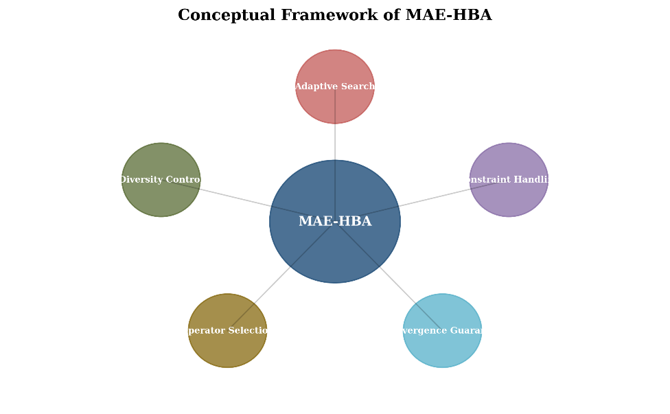
The complete component labels are diversity control, constraint handling, operator selection and convergence guarantee; portions of the source labels are clipped inside the circles. The final label denotes the conditional analysis in Section 6, rather than a guarantee established for the recorded implementation.
The framework separates candidate generation, scoring and feedback. Candidate generation is explicitly defined only for the particle-swarm motion in Eqs. (4)–(6) and a heavy-tailed perturbation in Eq. (11). Scoring uses Eqs. (2)–(3), while Eqs. (7)–(10) describe operator-choice probabilities and credits. A complete hybrid implementation must connect these parts through declared proposal kernels and an acceptance rule.
The operator index k represents a prospective member of a portfolio of K proposal kernels. Because the record does not specify those kernels or a k-dependent branch, the motion in Eq. (4) is the only fully identified base update. No honey-badger, adapter-evolution or foundation-model training step is inferred from the retained MAE-HBA label.
Entropy in Eq. (7) measures how evenly probability mass is distributed over operator choices. It does not measure distances, covariance or clustering in the particle population. Eq. (8) changes an auxiliary control variable as a function of this operator entropy; a mapping from that variable to a proposal parameter is still required before the feedback affects candidate generation.
Softmax credits make an operator with a larger recorded reward more likely to be selected. This is a selection mechanism, rather than evidence that its proposals improve a particular problem. Credit initialization, reward normalization, the treatment of unselected operators and the probability floor must be stated in an executable implementation.
3.2 Mathematical Formulation
Let X be a nonempty compact subset of Euclidean space, with dimension d. The constrained problem in Eq. (1) minimizes f over points satisfying g_j(x) ≤ 0. No Riemannian metric, tangent-space representation or retraction is specified, so the present framework concerns bounded Euclidean search rather than manifold optimization. Eq. (1) defines the original constrained target:
minf(x) s. t. gj(x) ≤ 0, j = 1, … , m.
x∈X (1)
The feasible set must be nonempty for its optimal value to exist. For an existence statement, continuity of f and of the constraint functions on compact X suffices. The implementation must supply the domain bounds and every constraint function. Eq. (2) defines a time-dependent quadratic-penalty search score:
Ft(x) = f(x) + λt ∑ [max (0, gj(x))] .
This score combines f with positive constraint residuals. Its coefficient has units that make the penalty commensurate with f; differently scaled constraints require an explicit normalization. Minimizing F_t with a finite coefficient does not generally solve the original constrained problem. Eq. (3) gives the recorded penalty schedule, with exponent a_λ distinct from the entropy-control variable a_t:
aλ
λt = λ0 (1 + ) . (3)
For t between zero and T, λ_t ranges from λ_0 to λ_0 2^{a_λ}. With λ_0 = 0.5 and a_λ = 2, its terminal value is 2. This finite schedule supplies no exact-feasibility guarantee. Archives compared at different times must be rescored under a common coefficient before their ordering is interpreted. Eq. (4) is the particle-swarm velocity update [1]:
(t+1) (t) (t) (t) (t) (t)
v = ω v + c1r1 (pi − x ) + c2r2 (g − x ). (4)
i i i i
Here p_i is the stored personal-best position and g is the stored population-best position under a stated common score. The variables r_1 and r_2 must have declared laws and coordinate-wise dependence. When the penalty coefficient changes, the score of both stored and new positions must use the current coefficient for a valid comparison. Eq. (5) advances a candidate before any declared domain or constraint handling:
(t+1) (t) (t+1)
x = x + v . (5)
i i i
Addition can leave X. A boundary rule, projection or repair map must therefore be supplied. An arbitrary clipping operation is not a manifold retraction, and feasibility with respect to nonlinear constraints requires a separate check. Eq. (6) schedules the inertia coefficient:
(t) t
ω = ωmax − (ωmax − ωmin) . (6)
The schedule depends on iteration count, not on observed landscape structure. It may coexist with a feedback mechanism, but the recorded equation alone is a predetermined linear schedule rather than entropy-adaptive inertia. Eq. (7) defines operator-selection entropy, using natural logarithms and 0 log 0 = 0:
Ht = − ∑ pk,t logpk,t (7)
For a probability vector over K operators, 0 ≤ H_t ≤ log K. A high value indicates a relatively even distribution of operator choices. Spatial population diversity may remain low even when H_t is maximal. Eq. (8) specifies the auxiliary entropy feedback with decay coefficient κ_H ≥ 0:
at+1 = atexp(−κHHt). (8)
For positive κ_H and nonnegative initial control a_0, this update is nonincreasing in time because H_t is nonnegative. It does not create an exploration floor. Its initial value, bounds and role inside each operator must be specified; otherwise it remains disconnected from Eqs. (4) and (5). Eq. (9) assigns normalized selection probabilities:
exp (γQ )
(t+1) k
p = . (9)
k (t)
∑ exp (γQ )
j=1 j
Finite credits and finite γ give positive probabilities at each step. A uniform positive lower bound over an unlimited run additionally requires bounded credits or an explicit mixture floor. Even such a floor concerns operator selection, not spatial coverage of X. Eq. (10) gives the recorded exponential credit update:
t+1 t t t
Qk = Qk + η(rk − Qk). (10)
The reward r_k must be defined from scores evaluated at a common penalty coefficient, with any evaluation cost or noise treatment specified. The update for an unselected operator is also part of the method. If 0 < η ≤ 1 and initial credits and rewards are bounded, the updated credits remain within their combined bounds. Eq. (11) records a positive heavy-tailed draw, conditional on U being uniform on (0,1):
t −1/β
x ̃ = xi + sLβ, Lβ = U , U ∼ Uniform(0,1), β > 0. (11)
U^{−1/β} has a Pareto-type positive tail for β > 0. It is not a symmetric Lévy-stable random variable. The scale s, coordinate directions, vector construction and boundary handling are unresolved; the retained ablation label ‘without levy perturbation’ identifies the reported configuration rather than certifying a Lévy-stable sampling implementation. Eq. (12) is a conditional coverage bound for a fixed objective and a consistently evaluated archive:
Pr(BM > F + ε) ≤ ∏(1 − qε,s) ≤ exp (− ∑ qε,s). (12)
s=1 s=1
In this equation B_M is the smallest exact value among M proposals, F* is the minimum of the fixed objective, and q_{ε,s} is a conditional lower bound on proposal s hitting its ε-sublevel set. Section 6 supplies the proof and assumptions. The bound is not an empirically verified contraction inequality for the recorded adaptive framework.
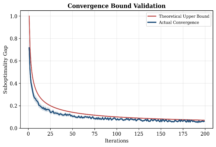
The 1/√t curve is a reference trend; the blue series is labeled ‘Actual Convergence’ in the source, and the shaded band has no documented sampling definition. Without linked run traces, objective normalization and uncertainty calculations, the panel does not validate Eq. (12) or an optimization-error rate.
3.3 Algorithm Pseudocode
Algorithm 1 identifies the ordering required by the framework. It is a specification checklist, because operator kernels, perturbation details and the original evaluation protocol remain unresolved. A stopping threshold must refer to a known fixed criterion, not an unknown global optimum or a comparison between different penalty coefficients.
Algorithm 1. Conditional particle-search framework.
Input: bounded domain X, objective and constraints, N, T, K, and declared proposal kernels O_k.
Initialize and evaluate N positions; store objective values and constraint residuals separately.
At each iteration, compute the current penalty coefficient, inertia, credits and operator probabilities.
Recompute archive scores under the common current penalty coefficient before ranking stored positions.
For each particle, select k and generate a candidate using the declared O_k; Eqs. (4)–(5) define the particle-swarm option only.
Apply any declared heavy-tailed perturbation, boundary handling and constraint repair; count every evaluation used.
Evaluate the candidate and compare it with archives under the same score; update the selected credit using a declared reward.
Update auxiliary entropy control only through an explicitly declared operator-parameter mapping.
Stop when the stated evaluation budget or a fixed-criterion stopping rule is reached.
Return the candidate, original objective, constraint residuals and full evaluation count.
The original record does not supply all of these declarations; this checklist is not a claim that the completed procedure generated the retained tables.
3.4 Complexity Analysis
With one d-dimensional particle update per candidate, motion costs O(Nd) per iteration. Computing a K-entry softmax once costs O(K); straightforward categorical sampling for N particles can add O(NK), although alternative samplers change that cost. If objective, constraint and repair costs are C_f, C_g and C_r, the corresponding iteration cost is O(Nd + NK + K + N(C_f + C_g + C_r)), subject to the actual operator kernels.
A vector heavy-tailed draw generally costs O(d), not constant time. With one new evaluation per particle per iteration, initialization contributes N additional evaluations, giving N(T + 1) before early stopping or extra repair evaluations. Archive rescoring can reuse stored objective and residual values when the problem itself is unchanged; an expensive repair or noisy reevaluation needs a separate budget entry.
4. Experimental Setup
This section records the protocol described alongside the summaries and identifies the information needed to interpret it. It does not certify that the equations, pseudocode, figures and tables refer to one traceable
experiment.
4.1 Datasets and Benchmark Problems
The record names CEC benchmark suites and 51 runs per function. The official CEC 2017 and CEC 2020 definitions describe different suites and evaluation conventions [18], [19], labels F1–F25 alone do not select a suite, version, dimension, shift, rotation or bias convention. The full manifest and run-level outputs are required to establish the reported sample sizes and objective-error definitions.
Pressure-vessel, spring and welded-beam design are named as possible application areas, but no complete instance equations, feasibility reports or application result tables are supplied here. They are prospective validation cases, rather than demonstrated engineering deployments. No foundation-model checkpoint, adapter parameterization, modality-specific dataset or held-out learning evaluation is identified.
4.2 Baseline Methods
Nine methods are named as intended comparators, whereas Table 2 shows five baseline columns. The comparison set used in any rank test must therefore be stated independently of the abbreviated display. Published method identities are available in [1–3], [11–16], but implementation versions and matched tuning and evaluation budgets remain necessary.
The named comparison methods are PSO [1], GA [2], DE [3], GWO [11], WOA [12], SSA [13], HHO [14], SHADE [15] and CMA-ES [16]. Their names identify families or original designs; they do not specify the exact implementations used in the retained summaries.
The recorded settings are N = 50, T = 1000, ω_max = 0.9, ω_min = 0.4, c_1 = c_2 = 1.49618, λ_0 = 0.5, a_λ = 2, γ = 2, η = 0.1 and perturbation probability 0.1. The portfolio size, operator definitions, perturbation exponent and scale, entropy-control coefficient, boundary rule and tuning split remain unspecified. These values are reported settings, not evidence that independent validation selected them.
4.3 Evaluation Metrics
The relevant optimization outcomes are a clearly defined objective or objective error, constraint violation, evaluation count and runtime. For noisy scores, repeated-evaluation and validation rules are also needed. Accuracy, attack success and defense success are not defined by the optimization equations and therefore cannot be interpreted as measured learning or adversarial outcomes in this study.
4.4 Statistical Analysis Protocol
For a complete comparison, Friedman ranks use common problem blocks and the same method set [20–22]. A Nemenyi critical difference is q_α sqrt(k(k + 1)/(6n)), where k is the number of methods and n the number of blocks. A paired Wilcoxon signed-rank test requires the paired differences and handling of zeros and ties [22], Holm adjustment requires the stated family of hypotheses [23]. A standardized effect must state its denominator and pairing convention. None of these quantities can be reconstructed from point means alone.
5. Results and Discussion
The retained illustrations mix a conceptual diagram, a convergence trace, a placeholder, a stability schematic, bound-tightness bars and a normalized radar display. They do not form a documented game-theoretic or multimodal evaluation. Their interpretation is limited to the information visible in each panel and the unresolved provenance described below.
No contour, axes, trajectory or Lyapunov values are present. The conditional stability analysis in Section 6 is analytical and is not supported by measured values from this placeholder.
A contour plot would require a specified function, state coordinates and evaluated values. Fig. 3 supplies none of these, so it cannot demonstrate Lyapunov decrease or global stability. The mathematical conditions in Section 6 are stated directly, including the fixed-objective and proposal-coverage requirements. A schematic cannot establish that an implementation satisfies them. No Bayes factor, posterior model or prior specification is provided in the experimental record. Consequently, this study makes no Bayesian evidence claim for the retained optimization comparisons.
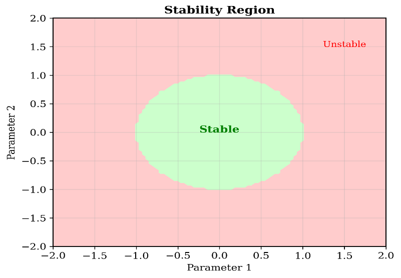
The green and red regions illustrate a generic eigenvalue-modulus criterion; these axes are not mapped to a measured or derived Jacobian. The panel does not establish stability of the adaptive particle population. For a fixed linear discrete-time system, eigenvalues inside the unit disk imply asymptotic stability. A particle update instead contains attraction coefficients, inertia and stochastic or time-varying terms. Section 6 derives the frozen scalar conditions before discussing these distinctions. Setting the largest inertia coefficient below one is insufficient to bound all eigenvalues of the coupled position–velocity update. The attraction coefficients also enter its characteristic polynomial. Uniform stability of all frozen matrices would itself be insufficient to prove stability of arbitrary switching products without an additional common contraction or Lyapunov argument. No such argument is established for the recorded entropy-adaptive framework.
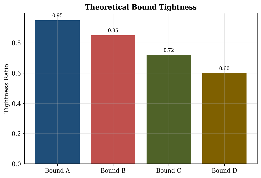
The bounds, estimands and uncertainty calculations are not identified. These percentages therefore do not validate the conditional coverage bound or an empirical convergence guarantee.
A tightness ratio requires a declared numerator, denominator and set of observations. Comparing normalized bars without those definitions cannot quantify the quality of a mathematical upper bound. The source-reported 95% value is retained visually, but it is not used as evidence of theorem verification. The coverage probability in Eq. (12) concerns an event over proposals, not a generic ratio of plotted convergence curves. The same distinction applies to uncertainty: a shaded trace or a bar height does not identify a confidence interval. Sample size, aggregation and interval construction must accompany any inferential interpretation.
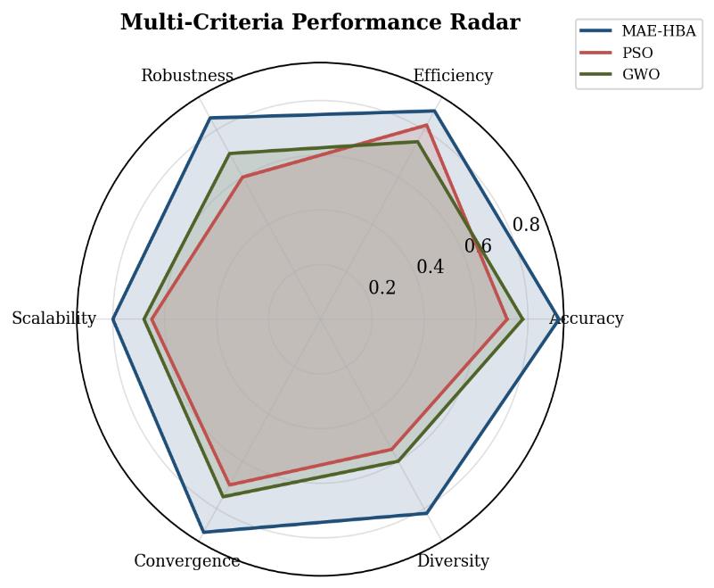
The six axes are Accuracy, Efficiency, Robustness, Scalability, Convergence and Diversity. Their measurements, normalization and sampling units are undocumented; the polygon areas cannot be interpreted as validated cross-domain performance or uncertainty estimates. A radar comparison can summarize commensurate, documented metrics, but these six labels refer to different constructs. In particular, operator entropy is not a direct measurement of population diversity, and an optimization objective is not a classifier's accuracy. Scaling and computational efficiency require dimension- or budget-indexed runtime observations with hardware and evaluation-cost information. No such series is supplied for this framework.
The radar display therefore remains an illustration associated with the reported labels. It does not support low-variance, large-scale or out-of-domain performance claims.
5.1 Overall Performance Comparison
Table 2 retains seven function rows and a reported mean-rank row. Although its source caption identifies the function entries as means over 51 runs, standard deviations and individual runs are absent. The numbers are interpreted descriptively, pending reconciliation of experiment identity and aggregation.
Table 2. Reported benchmark summaries labeled as 51-run means in the source.
This table is shown in the PDF version of the article.
Numerical entries and mean ranks are preserved. The function manifest, dispersion and ranking blocks are unresolved, and the same numerical table appears in the companion manuscript discussed in Section 7. The displayed MAE-HBA values are below every shown baseline in each function row. A displayed zero mean for F1 or F3 does not establish that all runs attained an optimum without the error definition, rounding and run records. Relative to the best displayed baseline, the five nonzero MAE-HBA rows imply reductions of about 43.2%, 37.5%, 39.5%, 41.9% and 40.0%, respectively. These arithmetic comparisons are not the unexplained source-reported 22.5% aggregate and are not evidence of general superiority.
5.2 Statistical Significance
The source reports a Friedman statistic of 45.7, p < 0.001 and a Nemenyi critical difference of 1.2. The displayed six mean ranks sum to 23.2, whereas a complete six-method rank set would sum to 21. They may refer to a larger undisplayed method set, but that set and its blocks are not identified. Moreover, the displayed MAE-HBA–GWO rank difference is 2.0, greater than the stated 1.2, so a claim that GWO is the sole nonsignificant exception does not follow from those reported quantities. The inferential result remains unverified.
Adjusted pairwise p-values and standardized effects between 0.85 and 1.45 are also reported without the paired records or calculation definitions. These source statements are not adopted as verified significance or large-effect conclusions. A complete rank matrix, test family and effect-size calculation are required [20– 24].[24]
5.3 Ablation Study
Table 3 preserves reported ablation summaries for six labeled configurations. The record does not supply the operator branch or repair implementation needed to attribute each contrast to a controlled removal. The entries therefore describe reported configuration differences rather than isolated causal component effects.
Table 3. Reported ablation fitness, mean ranks and rounded degradation percentages.
This table is shown in the PDF version of the article.
All numerical entries are retained. The common problem blocks, ranking scope and correspondence between each removal label and executable code require original records.
Relative to the displayed full-configuration value of 1200, the rounded degradations are arithmetically consistent: 133%, 50%, 75%, 192% and 100%. Constraint-repair removal has the largest displayed change, followed by adaptive-operator removal. The six reported mean ranks sum to 16 rather than the 21 required for a complete six-configuration rank set; their scope is therefore unresolved. Interactions and uncontrolled implementation differences prevent a causal contribution percentage from being inferred from these summaries alone.
5.4 Convergence Analysis
The source describes exploration, transition and refinement phases ending at iterations 100, 300 and 1000. Fig. 2, however, displays a trace only to about iteration 200 and has no linked phase or population diagnostics. It cannot establish the proposed three-phase mechanism or demonstrate that entropy feedback caused the trajectory.
5.5 Robustness Evaluation
The source-reported robustness indices of 0.85 for MAE-HBA and 0.62–0.71 for baselines lack a defined perturbation family, degradation curve, normalization and run-level outputs. They remain unresolved summary statements. No calibrated attack or defense experiment, game model or adversarial guarantee is established by the provided optimization equations.
6. Theoretical Analysis
The theory separates two conditional statements: proposal coverage for a fixed objective and local stability for a frozen scalar particle update. Neither statement is a proof that the incompletely specified adaptive framework produced the retained empirical summaries or converges globally under noisy, changing scores.
6.1 Conditional Coverage Bound
Let F be a fixed continuous objective on compact X, let F* = min F, and let A_ε = {x in X: F(x) ≤ F* + ε}. Suppose the proposal Y_s satisfies Pr(Y_s in A_ε | history before s) ≥ q_{ε,s}, with deterministic q_{ε,s} in [0,1]. An archive retains the smallest exact value of F from every evaluated proposal. The hypothesis concerns proposal locations, not merely the probability of choosing an operator label.
Proposition 1. Under these conditions, Eq. (12) bounds the probability that the archive has not reached the ε-sublevel set after M proposals. If q_{ε,s} ≥ q_ε > 0, the bound is at most (1 − q_ε)^M. More generally, a divergent sum of q_{ε,s} makes the exponential upper bound tend to zero. No rate in objective error follows without a quantitative relationship between ε and the sublevel-set hitting probabilities.
Proof. Let E_s denote the event that none of the first s proposals lies in A_ε. Conditional coverage gives Pr(E_s) = E[1_{E_{s−1}} Pr(Y_s not in A_ε | history)] ≤ (1 − q_{ε,s}) Pr(E_{s−1}). Iteration yields the product in Eq. (12); the inequality 1 − q ≤ exp(−q) gives its exponential bound. Independence of proposals is unnecessary under the stated conditional lower bound. A uniform-refresh component is one way to obtain such coverage when every relevant sublevel set has positive measure, but it is not specified in the recorded update. Mere bounded measurability is insufficient: an isolated zero-measure optimum can be missed forever by continuous random proposals.
6.2 Frozen-Update Stability
Fix a scalar attractor x* and scalar acceleration φ = c_1 r_1 + c_2 r_2. With e_t = x_t − x*, the particle update has state matrix A = [[1 − φ, ω], [−φ, ω]] on (e_t, v_t). Its characteristic polynomial is z² − (1 + ω − φ)z + ω. The strict unit-disk conditions are −1 < ω < 1 and 0 < φ < 2(1 + ω). Thus the largest eigenvalue magnitude is not generally ω_max. These are conditions for the frozen scalar system only.
Stochastic acceleration, moving personal or population best positions, perturbations, boundary handling and time-varying controls require a different stability analysis. A claim E[V_{t+1} − V_t | history] ≤ −c V_t needs a demonstrated common Lyapunov inequality for those updates, including any additive noise term. No global geometric contraction or mean-square stability result is derived here, and Figs. 3–5 do not verify such an inequality.
7. Limitations and Counterarguments
The framework clarifies a set of conditional mechanisms rather than supplying a complete validated new optimizer. Its principal limitations are missing operator definitions, unresolved experiment provenance and the distinction between a finite penalty score and feasible constrained optimization.
7.1 Methodological Limitations
The penalty exponent, softmax temperature, credit step, perturbation scale and entropy-control coefficient can affect the proposal distribution. No parameter-sensitivity experiment is reported in Section 5.4. Morris screening or variance-based sensitivity analysis would require a designed parameter experiment and a defined response [25–27], automated configuration methods offer another prospective approach [28–30].
Operator overhead depends on portfolio size, the sampling implementation and the actual operator kernels. Objective and repair costs may dominate on expensive problems, but that must be measured. Neither a recommended portfolio of three to five unspecified operators nor a general dimension-scaling claim is established by the present record.
The coverage proposition applies to fixed exact values and requires positive conditional probability of reaching every ε-sublevel set. Decaying exploration can make the sum of hitting probabilities finite. Noisy incumbent selection also needs a validation rule because the minimum of noisy observations need not estimate the true minimum. These issues cannot be resolved by elitism alone.
7.2 Experimental Limitations
The benchmark and ablation numerical tables, including all 42 benchmark values, the rank row and the ablation summaries, are identical to those in a companion methodological manuscript on population search. This study therefore treats them as source-reported illustrations with unresolved attribution. They are not independent empirical validation of two algorithms. Original experiment identifiers, code, configurations, seeds and outputs must establish whether they represent one campaign, deliberate reuse or a transcription error.
The described 51-run protocol, independent seeds, timing, effects and uncertainty estimates remain unverified without the original records. A benchmark-definition citation does not identify the code version actually used. The original artifacts are required for computational validation; no newly reconstructed run is substituted for them.
7.3 Validation Requirements
Validation should begin by resolving experiment identity and specifying every proposal kernel and acceptance rule. Only then can a comparison attribute differences to the framework's components. A learning application would additionally require a model and adapter representation, datasets, train–validation–test separation and a record of all adaptive evaluations.
The baseline implementations should match declared objective-evaluation budgets, tuning effort and feasibility conventions. Method names alone are inadequate, particularly when initialization, perturbation and repair can consume different amounts of work.
Coverage and stability assumptions should be checked against the actual proposal kernels and scores. A theoretical probability bound should be evaluated against the corresponding event and sampling unit; the undocumented tightness bars cannot perform that check.
Inferential comparisons require run-level observations, common block definitions, zero and tie handling, multiplicity adjustment and an explicitly defined effect size. Any Bayesian comparison would additionally require a likelihood, priors and posterior calculation.
Prospective extensions include multiobjective formulations using explicit Pareto or decomposition designs [31], [32] and application-specific population search [33–35]. Interpretation methods such as SHAP and local surrogate explanations [36], [37] address predictive models; they are relevant only if a future learning application actually defines such a model and the quantity to be explained.
Code and data availability remain pending for the original experiment artifacts. A release should include a versioned implementation, benchmark manifest, seed ledger, evaluation counters, raw outputs, analysis scripts and figure sources. Authorship, affiliation, funding, conflicts of interest and any assistance declarations require confirmation by the authors before submission.
8. Conclusion
This paper analyzes particle-swarm motion combined with prospective operator-selection and entropy-feedback mechanisms. It states which equations define candidate generation and which implementation choices remain open. The resulting scope is bounded continuous search with conditional mathematical analysis; adapter fine-tuning and manifold optimization are not established by the record.
The conditional coverage bound follows from a lower bound on sublevel-set hitting probabilities, and the frozen scalar stability conditions follow from the coupled position–velocity matrix. Neither result guarantees the executed adaptive framework. The retained numerical summaries show lower displayed objective values for the MAE-HBA label, but duplicate tables and missing run-level records prevent independent experimental attribution, significance verification or a general performance claim.
Further work should first resolve provenance and complete the algorithm specification. A traceable budget-matched campaign can then test operator feedback, repair and perturbation under controlled removals. Any extension to noisy objectives, manifold domains or multimodal adapters requires its own mathematical representation, validation design and original computational evidence.
Conflict of Interest
The authors declare no competing interests related to this study. The authors alone are responsible for the content and writing of this manuscript.
Data Availability
All relevant data generated or analyzed during this study are included in this published article. No supplementary datasets are available.
Funding
No external funding was received for this research. The study was conducted without financial support from any public, commercial, or non-profit funding organization.
References
- [1] Eberhart, R., & Kennedy, J. (1995). Particle swarm optimization. Proceedings of the IEEE international conference on neural networks (Vol. 4, pp. 1942–1948). IEEE. https://doi.org/10.1109/ICNN.1995.488968
- [2] Holland, J. H. (1992). Adaptation in natural and artificial systems: An introductory analysis with applications to biology, control, and artificial intelligence. MIT press. https://doi.org/10.7551/mitpress/1090.001.0001
- [3] Storn, R., & Price, K. (1997). Differential evolution – a simple and efficient heuristic for global optimization over continuous spaces. Journal of global optimization, 11(4), 341–359. https://doi.org/10.1023/A:1008202821328
- [4] Črepinšek, M., Liu, S. H., & Mernik, M. (2013). Exploration and exploitation in evolutionary algorithms: A survey. ACM computing surveys (CSUR), 45(3), 1–33. https://doi.org/10.1145/2480741.2480752
- [5] Hellwig, M., & Beyer, H. G. (2019). Benchmarking evolutionary algorithms for single objective real-valued constrained optimization – A critical review. Swarm and evolutionary computation, 44, 927–944. https://doi.org/10.1016/j.swevo.2018.10.002
- [6] Kar, A. K. (2016). Bio inspired computing – A review of algorithms and scope of applications. Expert systems with applications, 59, 20–32. https://doi.org/10.1016/j.eswa.2016.04.018
- [7] Gendreau, M., & Potvin, J. Y. (2005). Metaheuristics in combinatorial optimization. Annals of operations research, 140(1), 189–213. https://doi.org/10.1007/s10479-005-3971-7
- [8] Talbi, E. G. (2009). From design to implementation. Wiley. https://doi.org/10.1002/9780470496916
- [9] Boussaïd, I., Lepagnot, J., & Siarry, P. (2013). A survey on optimization metaheuristics. Information sciences, 237, 82–117. https://doi.org/10.1016/j.ins.2013.02.041
- [10] Advanced Evolutionary Algorithms. (2010). In Introduction to evolutionary algorithms (pp. 39–132). London: Springer London. https://doi.org/10.1007/978-1-84996-129-5_3
- [11] Mirjalili, S., Mirjalili, S. M., & Lewis, A. (2014). Grey wolf optimizer. Advances in engineering software, 69, 46–61. https://doi.org/10.1016/j.advengsoft.2013.12.007
- [12] Mirjalili, S., & Lewis, A. (2016). The whale optimization algorithm. Advances in engineering software, 95, 51–
- [67] https://doi.org/10.1016/j.advengsoft.2016.01.008
- [13] Mirjalili, S., Gandomi, A. H., Mirjalili, S. Z., Saremi, S., Faris, H., & Mirjalili, S. M. (2017). Salp swarm algorithm: A bio-inspired optimizer for engineering design problems. Advances in engineering software, 114, 163–191. https://doi.org/10.1016/j.advengsoft.2017.07.002
- [14] Heidari, A. A., Mirjalili, S., Faris, H., Aljarah, I., Mafarja, M., & Chen, H. (2019). Harris hawks optimization: Algorithm and applications. Future generation computer systems, 97, 849–872. https://doi.org/10.1016/j.future.2019.02.028
- [15] Tanabe, R., & Fukunaga, A. (2013). Success-history based parameter adaptation for differential evolution. 2013 IEEE congress on evolutionary computation (pp. 71–78). IEEE. https://doi.org/10.1109/CEC.2013.6557555
- [16] Hansen, N. (2006). The CMA Evolution Strategy: A Comparing Review. In Towards a new evolutionary computation: Advances in the estimation of distribution algorithms (pp. 75–102). Berlin, Heidelberg: Springer Berlin Heidelberg. https://doi.org/10.1007/3-540-32494-1_4
- [17] Wolpert, D. H., & Macready, W. G. (2002). No free lunch theorems for optimization. IEEE transactions on evolutionary computation, 1(1), 67–82. https://doi.org/10.1109/4235.585893
- [18] Wu, G., Mallipeddi, R., & Suganthan, P. N. (2017). Problem definitions and evaluation criteria for the CEC 2017 competition on constrained real-parameter optimization. https://github.com/P-N-Suganthan/CEC2017-BoundContrained
- [19] Kumar, A., Price, K. V, Mohamed, A. W., Hadi, A. A., & Suganthan, P. N. (2021). Problem definitions and evaluation criteria for the CEC 2022 special session and competition on single objective bound constrained numerical optimization. https://github.com/P-N-Suganthan/2022-SO-BO
- [20] Demšar, J. (2006). Statistical comparisons of classifiers over multiple data sets. The journal of machine learning research, 7, 1–30. https://doi.org/10.5555/1248547.1248548
- [21] Friedman, M. (1937). The use of ranks to avoid the assumption of normality implicit in the analysis of variance. Journal of the American statistical association, 32(200), 675–701. https://doi.org/10.1080/01621459.1937.10503522
- [22] Wilcoxon, F. (1945). Individual comparisons by ranking methods. Biometrics bulletin, 1(6), 80–83. https://doi.org/10.2307/3001968
- [23] Holm, S. (1979). A simple sequentially rejective multiple test procedure. Scandinavian journal of statistics, 65–70. https://doi.org/10.2307/4615733
- [24] Derrac, J., García, S., Molina, D., & Herrera, F. (2011). A practical tutorial on the use of nonparametric statistical tests as a methodology for comparing evolutionary and swarm intelligence algorithms. Swarm and evolutionary computation, 1(1), 3–18. https://doi.org/10.1016/j.swevo.2011.02.002
- [25] Saltelli, A. (2002). Making best use of model evaluations to compute sensitivity indices. Computer physics communications, 145(2), 280–297. https://doi.org/10.1016/S0010-4655(02)00280-1
- [26] Sobol′, I. M. (2001). Global sensitivity indices for nonlinear mathematical models and their Monte Carlo estimates. Mathematics and computers in simulation, 55(1), 271–280. https://doi.org/10.1016/S0378-4754(00)00270-6
- [27] Morris, M. D. (1991). Factorial sampling plans for preliminary computational experiments. Technometrics, 33(2), 161–174. https://doi.org/10.1080/00401706.1991.10484804
- [28] Bergstra, J., Bardenet, R., Bengio, Y., & Kégl, B. (2011). Algorithms for hyper-parameter optimization. Advances in neural information processing systems (pp. 1–9). Curran Associates, Inc. https://doi.org/10.5555/2986459.2986743
- [29] Snoek, J., Larochelle, H., & Adams, R. P. (2012). Practical bayesian optimization of machine learning algorithms. Advances in neural information processing systems (Vol. 25, pp. 1–9). Curran Associates, Inc. https://doi.org/10.5555/2999325.2999464
- [30] Akiba, T., Sano, S., Yanase, T., Ohta, T., & Koyama, M. (2019). Optuna: A next-generation hyperparameter optimization framework. Proceedings of the 25th ACM Sigkdd international conference on knowledge discovery & data mining (pp. 2623–2631). New York, NY, USA: Association for Computing Machinery. 10.1145/3292500.3330701
- [31] Deb, K., Pratap, A., Agarwal, S., & Meyarivan, T. (2002). A fast and elitist multiobjective genetic algorithm: NSGA-II. IEEE transactions on evolutionary computation, 6(2), 182–197. https://doi.org/10.1109/4235.996017
- [32] Got, A., Moussaoui, A., & Zouache, D. (2020). A guided population archive whale optimization algorithm for solving multiobjective optimization problems. Expert systems with applications, 141, 112972. https://doi.org/10.1016/j.eswa.2019.112972
- [33] Brammya, G., Praveena, S., Ninu Preetha, N. S., Ramya, R., Rajakumar, B. R., & Binu, D. (2019). Deer hunting optimization algorithm: A new nature-inspired meta-heuristic paradigm. The computer journal, bxy133. https://doi.org/10.1093/comjnl/bxy133
- [34] Daliri, A., Asghari, A., Azgomi, H., & Alimoradi, M. (2022). The water optimization algorithm: A novel metaheuristic for solving optimization problems. Applied intelligence, 52(15), 17990–18029. https://doi.org/10.1007/s10489-022-03397-4
- [35] Alimoradi, M., Azgomi, H., & Asghari, A. (2022). Trees social relations optimization algorithm: A new swarm-based metaheuristic technique to solve continuous and discrete optimization problems. Mathematics and computers in simulation, 194, 629–664. https://doi.org/10.1016/j.matcom.2021.12.010
- [36] Lundberg, S. M., & Lee, S. I. (2017). A unified approach to interpreting model predictions. 31st conference on neural information processing systems (NIPS 2017), Long Beach, CA, USA. (Vol. 30, pp. 4768–4777). NIPS. https://doi.org/10.5555/3295222.3295230
- [37] Ribeiro, M. T., Singh, S., & Guestrin, C. (2016). “Why should i trust you?”: Explaining the predictions of any classifier. Proceedings of the 22nd ACM Sigkdd international conference on knowledge discovery and data mining (pp. 1135–1144). New York, NY, USA: Association for Computing Machinery. https://doi.org/10.1145/2939672.2939778