Stochastic Global Search on Molecular Potential-Energy Surfaces: A Narrative Survey and a Reported Numerical Illustration

2.1 Population-Based Search on Clusters and Molecules

Population search varies ensembles of candidate coordinates or structural descriptors. Hartke’s phenotype algorithm with niches concerns cluster geometry [8], while Zhou, Zhao and Cheng develop a revised particle-swarm algorithm for cluster structure prediction [9]. CALYPSO provides a separate example of particle-swarm-based crystal structure prediction [18]. These studies support the relevance of population search to structural problems without proving a common failure mode for every DE, PSO, CMA-ES or GWO configuration. General constrained-surrogate studies [14], [15], [19] likewise concern computational search design, rather than ReaxFF fitting or validated molecular performance.

2.2 Basin-Hopping and Trajectory Methods

Basin hopping maps a candidate configuration to a locally minimized energy and explores the resulting basin representation [10], [11]. Minima hopping uses local relaxation with an adaptive escape and acceptance mechanism [12]. Rondina and Da Silva’s [20] revised basin-hopping study addresses clusters and nanoparticles. Carmona et al. [21] preprint describes adaptive and parallel basin hopping for Lennard-Jones clusters, including concurrent local minimizations it is a methods report rather than a literature review. The local solver, move distribution, acceptance rule and total parent evaluations remain essential parts of any comparison.

2.3 Surrogate-Assisted and ML-Potential Hybrids

Surrogate-assisted evolutionary computation uses approximate response models to reduce or redirect expensive fitness calls; model management is part of the optimization method [13]. Global/local collaboration and two-stage DE have been studied for general expensive constrained problems [14], [15], [19]. Direct chemistry examples have different models and tasks. Jung et al. [16] combine an on-the-fly Gaussian Approximation Potential with constrained minima hopping for surface adsorbate geometries and DFT refinement. Yang et al. [16] combine a deep neural network, transfer learning and a genetic algorithm for metal-cluster structures. These are relevant precedents for checked approximate energy models, rather than validation of the present GP integration sketch.

Machine-learned potentials also arise outside global geometry search. Behler and Parrinello [22] introduce a neural-network representation of potential-energy surfaces, and Chmiela et al. [23] develop energy-conserving molecular force fields.

Jinnouchi et al. [24] use on-the-fly force-field learning in molecular dynamics and melting-point calculations. Their settings illustrate model construction and parent-model checking, but do not imply a universal change from cubic DFT cost to quadratic potential cost. Replacing a GP with an interatomic potential requires suitable descriptors, symmetry handling, training data and extrapolation checks; it is not an interchangeable validated module.

2.4 Conformational Search and Crystal-Structure Prediction

Molecular conformer exploration and crystal structure prediction have related energy-search goals but distinct coordinate spaces and constraints. Pracht et al. [25] describe automated low-energy chemical-space exploration with fast quantum chemical methods.

CALYPSO combines particle-swarm search with structural-generation and diversity mechanisms [18], USPEX connects evolutionary search with ab initio total-energy calculations [26], and AIRSS uses random structure searching with first-principles relaxation [27]. These established approaches broaden the survey beyond isolated clusters. The numerical illustration below does not test conformer populations, variable crystal cells, surface coverage or electronic-method selection, so quantitative transfer to those tasks is not claimed.

2.5 Statistical Methodology in Algorithm Comparison

Algorithm comparison must distinguish independent problem instances from repeated stochastic searches on one instance. Nonparametric comparison methods and their assumptions are discussed by Derrac et al. [28], and Doye et al. [29]. Cliff’s delta compares two empirical distributions [30], whereas a paired signed-rank test uses within-pair differences. Hedges’ bias correction concerns standardized mean differences [31], and Morris screening concerns elementary effects under a specified sampling design [32]. No test name establishes the validity of missing input arrays, uncertain pairing or an unmatched cost budget.

Fig. 1 illustrates the conceptual distinction between exploring configurations and refining a basin. It is retained as a schematic, not an observed SAHS trajectory or a computed molecular potential. Without the underlying potential formula and stationary-point calculations, the marked minima and saddle cannot be verified from its colored surface alone.

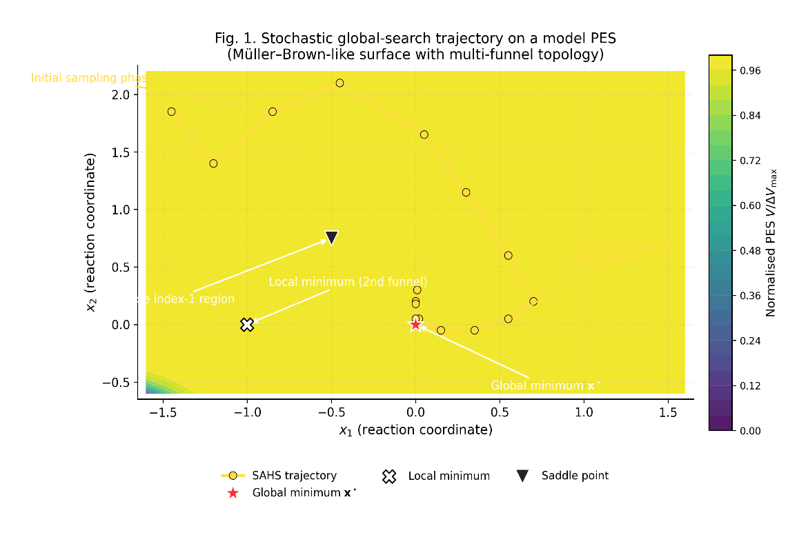
The trajectory and stationary-point labels are schematic; neither their coordinates nor the potential formula are supplied as a verified numerical experiment. The figure is not evidence that SAHS reached a global minimum.

3.1 Potential-Energy Surface and Stationary Points

An N-atom geometry can first be represented by Cartesian coordinates in R³ᴺ, with an admissible set that includes physical and numerical constraints. Removing rigid translations and rotations gives 3N − 6 local internal degrees of freedom for a nonlinear isolated geometry with N ≥ 3, and 3N − 5 for a linear geometry. The quotient has singular cases and need not be one global Euclidean coordinate chart. On a differentiable local representation, stationary points satisfy ∇V(x) = 0. A positive-definite Hessian is sufficient for a strict nondegenerate local minimum; a minimum can also have flat directions. The energy model, constraints and representation must remain fixed when comparing candidate energies [1], [2].

3.2 Multi-Funnel Topology

The LJ₃₈ example has a documented double-funnel landscape, with face-centered-cubic and competing icosahedral structural families [29]. The primary study supplies the landscape context and reduced Lennard-Jones units. It does not establish which basin any present run entered, and its known minimum transfers only when the potential definition and units match. Poor search performance alone does not demonstrate that a population collapsed into a particular structural family; that requires coordinates or structural classifications.

3.3 Saddle-Point Structure and Index

At a nondegenerate stationary point, the Hessian’s number of negative eigenvalues defines its saddle index. An index-one stationary point can represent a transition state when the relevant chemical and dynamical conditions hold [2], [3]. Degenerate stationary points require more than the Hessian signature. Local descent converges according to its starting point and basin geometry; it need not end at the Euclidean-nearest local minimum. Global-search methods use stochastic moves, diverse proposals or escape mechanisms to explore additional basins, without providing a general finite-budget guarantee of finding the global minimum.

3.4 Cost-Aware Optimisation Statement

A cost-aware statement should describe a search policy π that generates evaluated configurations x₁,…,x_T from available information. Let X_obs(π) be its nonempty set of admissible configurations evaluated by the parent model, and let c_work(x_t) denote serial computational work in seconds per parent call. Eq. (1) defines the final observed recommendation and a work budget. If the resource is instead call count, set c_work = 1 and express B in calls; the two budgets must not be mixed.

x ̂π ∈ arg min V(x), ∑ cwork (xt) ≤ B. (1)

x∈ obs(π)

3.5 Cost Model and Kernel Selection

Electronic-structure evaluation cost depends on the method, basis or grid, SCF convergence, gradients and implementation [2]. Conventional scaling statements refer to specified computational representations and algorithms, not universal thresholds in the number of atoms. There is no universal twenty-five-atom limit for coupled-cluster calculations. Semi-empirical, DFT and correlated wave-function models also provide different energy approximations; cheaper evaluation is not equivalent to preserving the target landscape. The source’s PBE/TZVP timing calibration is a reported assumption for its synthetic illustration, rather than a documented series of PBE/TZVP geometry calculations.

A sum of serial call costs is total work, not parallel wall time. Parallel elapsed time additionally depends on task scheduling, concurrent occupancy, synchronization, local minimization and model-fitting overhead. Minimum interatomic distances, boundaries and other admissibility conditions belong in the evaluation protocol. Reporting total parent calls, function and gradient work, and elapsed time separately is necessary to assess a claimed cost–accuracy trade-off.

4.1 Algorithm Sketch

SAHS combines a DE-style population, a GP surrogate, locally relaxed basin-hopping proposals and Lévy perturbations associated with a diversity threshold. The source also reports an adaptive operator-portfolio ablation, although the operator choices and probability-update rule are absent from the sketch. Table 1 retains its numerical settings and ranges. These descriptions identify components but do not define a complete executable algorithm or establish that every described component was present in the reported runs.

F is the DE mutation scale, distinct from crossover probability CR; N_pop is population size, distinct from atom count. The values are retained and their executed implementation requires confirmation.

4.2 Algorithmic Components

The DE/rand/1 backbone uses mutation and binomial crossover [4]. The GP predicts an energy mean μ̂ and predictive standard deviation σ̂ in energy units. Maximizing a(x) = −μ̂(x) + λ_s σ̂(x) is equivalent to minimizing the lower-confidence score μ̂(x) − λ_s σ̂(x), for nonnegative dimensionless λ_s. This is an exploration heuristic, not an upper-energy minimization rule or a certified energy error bound. The source assigns a local-search probability p_LS, Lévy stability α and diversity threshold ρ, but the relationship between candidate selection, true evaluation and local relaxation requires the original implementation.

4.3 Pseudocode Sketch

The reported sequence initializes sixty candidate geometries and evaluates the parent potential, fits the GP, creates DE proposals, scores them, selects candidates and evaluates those passing an improvement gate. A local-relaxation step may follow, and low diversity may trigger a perturbation of the bottom thirty percent of the population. Re-evaluation of the population is reported every K = 20 iterations. The gate’s incumbent, score scale, candidate count, acceptance ordering, repair rule and portfolio update remain unspecified. Every new parent and gradient calculation in these steps must enter the same resource accounting; surrogate scores are not parent observations.

4.4 Cost Budget Allocation

Periodic parent-model checks can detect prediction error at the configurations checked. They do not guarantee that approximate predictions contain no false minima, nor prevent all extrapolation errors between checks. The source describes an improvement threshold ε = 10⁻⁴, but its objective units and exact comparison rule are needed to interpret the gate. The surrogate weight λ_s does not by its definition determine gating accuracy. Preliminary false-minimum trials and robust behavior under model misspecification are not independently documented by the retained summaries.

4.5 Surrogate Model Details

The reported GP uses a Matérn-5/2 ARD kernel and marginal-likelihood optimization by L-BFGS-B with five restarts. The description simultaneously refers to all evaluated points, training sizes of thirty to one hundred, and eighty selected or inducing points. Subset-of-data fitting and inducing-point approximation are different procedures, and eighty selected points cannot be used from a smaller dataset without a different convention. These alternatives must be resolved from the code. Population-based whitening likewise requires the same transform for stored training points and proposals, with refitting or consistent remapping whenever the transform changes; its numerical benefit is not measured in the retained record.

5.1 Benchmarks

The source reports an LJ₃₈ illustration and thirty distinct synthetic potential functions sampled from a Gaussian random field with anisotropic length scales and nonstationary noise. It separately reports thirty search seeds. The function archive and aggregation rules are needed to distinguish function-level blocks from seed-level runs and to identify whether the designs were fully crossed. The synthetic functions are not electronic-structure surfaces computed by HF, DFT or CCSD(T). Their stated 22-second PBE/TZVP-equivalent calibration requires a reference calculation and timing log. LJ energies should be reported in reduced ε units unless an explicit conversion is supplied [29]. Negative retained differences are therefore treated below as signed differences from an unverified stated reference, not certified gaps to a true global minimum.

5.2 Algorithms and Baselines

The reported comparison includes DE, PSO, CMA-ES, GWO, BH and SAHS, with population size sixty and four hundred iterations. The product 400 × 60 = 24,000 is a proposal-iteration count under a full-population interpretation, not a verified total of parent evaluations. The source reports up to two hundred L-BFGS steps after accepted moves; function calls, gradient calls and any numerical-difference evaluations must also be counted. Population wrappers for BH, restart counts, surrogate calls and shared initialization need explicit conventions before an equal-cost or equal-evaluation comparison can be established.

5.3 Hardware and Seeds

The source identifies a dual-socket Xeon Gold 6248R system, 384 GB RAM, Ubuntu 22.04, and a sixteen-core, 64 GB assignment per configuration. Its phrase “48 logical cores” is retained only as a source hardware description requiring confirmation. Seeds 1001–1030 and master seed 20240901 are reported, but the exact generator, stream allocation and function/seed pairing require the run records. Seed labels alone do not establish statistical independence or common starting geometries. The reported elapsed times include local minimization and exclude disk I/O; no independent timing reproduction is claimed.

5.4 Surrogate and Population Hyperparameters

Reported baseline settings are DE F = 0.5 and CR = 0.9 with crossover jitter ±0.1, PSO inertia decreasing from 0.7 to 0.4 with c₁ = c₂ = 1.5, CMA-ES initial step size 0.3 with up to three IPOP restarts, and linearly decreasing GWO parameter a. BH’s stated Gaussian step 0.4 Å and temperature parameter 0.5 eV, together with gradient tolerance 10⁻⁶ Hartree/Bohr, cannot be applied unmodified to reduced-unit LJ energies. A consistent coordinate and energy conversion, or separate settings per task, is needed. Table 1 and K = 20 retain the reported SAHS numerical parameters without certifying their execution.

5.5 Statistical Protocol

The source reports median and interquartile summaries, paired signed-rank tests with Holm correction over five contrasts, Cliff’s delta, Hedges’ g with BCa intervals, a Friedman/Nemenyi analysis on thirty function blocks, and Morris screening of six settings. Its methods specify 5,000 bootstrap resamples; the abstract’s former 10,000 claim is not used. The metric arrays, zero/tie treatment, exact or approximate test implementation, bootstrap resampling unit and correction family are required to reproduce these outputs. SciPy is a reported software context [33], not evidence that a particular statistical calculation was executed correctly. No new optimization campaign or bootstrap rerun is presented in this survey.

6.1 Reported LJ₃₈ Convergence

Fig. 2 preserves the source convergence curves and annotations. A fixed set of minimization runs has a nonincreasing best-so-far value in each run, and its pointwise median is also nonincreasing. Several displayed traces rise, so the plotted statistic cannot be certified as that fixed-run median without the original traces and aggregation code. The annotated iteration-80 and iteration-110 entries do not independently establish arrival in a global funnel; their plotted energy differences are not zero and basin identity requires structural information. No mechanistic explanation is inferred from a curve inflection alone.

The source does not provide a trace-level record linking surrogate fitting, local relaxation, basin identity or restart events to these plotted curves. Consequently, the curves support only a visual record of the reported illustration. They do not measure the causal contribution of the GP or establish a diagnostic threshold for selecting λ_s on a new molecular problem.

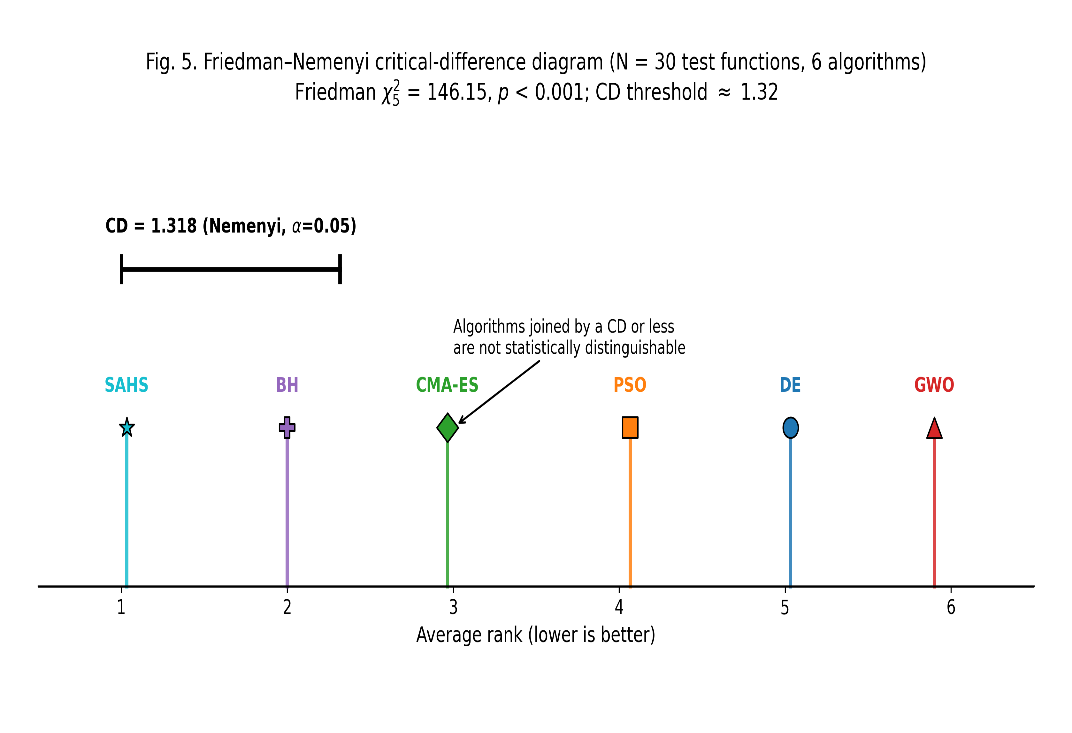
The source labels the lines as medians and bands as 25–75% ranges over thirty seeds. Upward changes conflict with fixed-run best-so-far minimization summaries; original traces, aggregation and reference definitions are required. The embedded basin-entry annotations are unverified.

6.2 Friedman–Nemenyi Analysis on 30 Functions

The source reports Friedman χ² = 146.15 with five degrees of freedom across thirty function blocks, giving an asymptotic chi-square tail of approximately 8.81 × 10⁻³⁰. The reported mean ranks are SAHS 1.03, BH 2.00, CMA-ES 2.97, PSO 4.07, DE 5.03 and GWO 5.90. These rounded ranks sum to twenty-one but do not independently reproduce the statistic or its tie correction. Using the conventional Nemenyi value q₀.₀₅ = 2.850 for six methods [34], CD = 2.850√[6 × 7/(6 × 30)] ≈ 1.377, not 1.318. The displayed SAHS–BH rank distance 0.97 is below this corrected threshold; the other SAHS distances exceed it. This conditional arithmetic check does not establish the original block-level analysis or equivalence with BH.

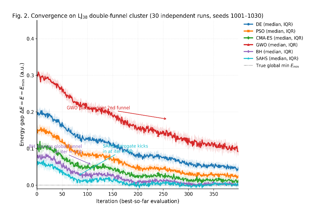
The embedded CD = 1.318 annotation is retained as a historical source label; conventional six-method, thirty-block Nemenyi arithmetic gives approximately 1.377. Original function-level ranks and the plotting settings are required to regenerate the diagram. A nonsignificant contrast does not demonstrate equivalence.

6.3 Cost Portfolio and Wall-Clock

Fig. 4 reports count and elapsed-time summaries, including approximately 3,600 parent-labeled evaluations and 295 seconds for SAHS. These labels require task-specific accounting. If each of 3,600 calls actually consumed twenty-two serial seconds and at most sixteen calls ran concurrently, their work alone would require at least 3,600 × 22/16 = 4,950 elapsed seconds under ideal full occupancy, before other work. This conflicts with 295 seconds under that interpretation. Synthetic timing, cache hits, internal kernel parallelism or a different counter definition cannot be assumed as the resolution without logs. The preserved plot therefore does not establish a production-DFT speed-up or matched parent-work savings.

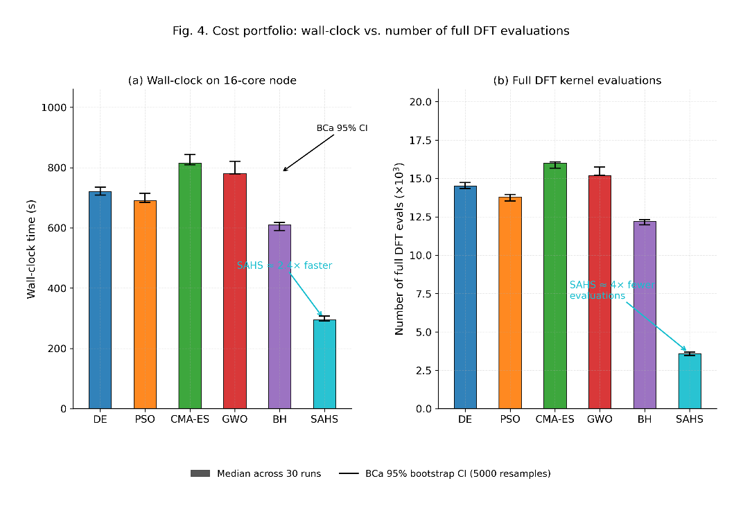
“DFT” is the source counter label, not a verified series of electronic-structure calls. The twenty-two-second calibration, sixteen-core assignment and 295-second summary require reconciliation. The source reports 5,000-resample BCa intervals; raw timing and count arrays are needed to verify them.

6.4 Ablation of Algorithmic Components

Table 2 preserves the component summaries. Disabling the GP changes the reported count from 3,600 to 14,200, a ratio of 3.94 and a reduction of 74.65 percent relative to the no-GP count. The accuracy entries also change from 0.0000 to 0.0050, so this is not a comparison at exactly matched accuracy. Disabling local search changes the displayed accuracy to 0.0120 and elapsed time to 320 seconds, an increase of 25 seconds or 8.47 percent. Original variant logs and matched histories are required to establish what was changed and how costs were charged.

The no-Lévy entry is 0.0080 rather than 0.0000, contradicting an assertion of unchanged median accuracy. Disabling the operator portfolio gives 0.0150 and 312 seconds, differences of 0.0150 and seventeen seconds from the full row. Disabling diversity restart gives 0.0220 and 338 seconds. These numerical contrasts do not imply additive or uniquely causal component effects: disabling one component changes the subsequent search history. The table contains no variant interquartile spans, so a thirty-percent variance-reduction claim cannot be obtained from it.

Original numeric cells are retained; the ΔE header is typographically normalized. Accuracy entries require the stated reference and units; the “DFT” counter requires an executed-work definition. These are reported contrasts, not newly reproduced ablations or certified matched-accuracy comparisons.

6.5 Run-to-Run Variability

Table 3 preserves the reported final signed-difference distributions. SAHS has Q25 = −0.0046 and Q75 = 0.0020, an interquartile span of 0.0066; the corresponding spans are 0.0099 for BH, 0.0136 for CMA-ES, 0.0249 for PSO, 0.0279 for DE and 0.0201 for GWO. These are arithmetic differences of displayed quartiles. A true gap E − E_global for the same exact potential cannot be negative; values such as −0.0046 require a matched reference, energy convention and calculation record. Finite-precision noise is not an established explanation. The summaries do not certify a basin or guarantee the quality of a future single run. The source’s atomic-unit interpretation and negative global-gap interpretation are unresolved; reduced-unit LJ requires an explicit conversion before physical energy units can be assigned.

6.6 Population Diversity

Fig. 3 shows the source population-diversity traces for DE, PSO and CMA-ES. A mean pairwise Euclidean distance depends on coordinate units, alignment, representation and population size. It does not by itself measure exploration of different structural basins or conversion of exploration into objective improvement. Source trace arrays and the normalization rule are required to verify the stated aggregation and relate diversity to an identified basin.

No SAHS diversity trace accompanies the preserved figure, so the assertion that it lies between the displayed extremes is not established. Neither a universal diversity threshold of one nor collapse within fifty iterations supplies a task-independent failure criterion. Diversity can be a diagnostic only when its representation and relationship to subsequent parent-model outcomes are specified.

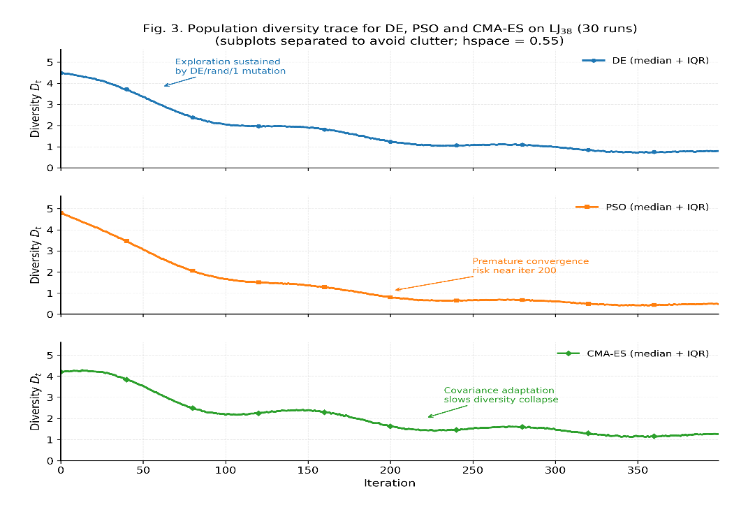
The source reports mean pairwise Euclidean distance and thirty-run aggregation; the median/IQR labeling and normalization require original arrays and plotting code. No SAHS trace is shown, and a structural-basin classification is not supplied.

6.7 Paired Statistical Tests

Table 4 preserves the paired-test and effect-size entries. The displayed Holm values are below 0.05 for DE, PSO, CMA-ES and GWO and above 0.05 for BH; these are reported significance decisions pending the original paired arrays and test specification. For thirty nonzero differences under exact two-sided sign randomization, the smallest attainable p-value is 2/2³⁰ ≈ 1.86265 × 10⁻⁹. The GWO entry 9.31 × 10⁻¹⁰ is below that minimum, and may reflect a different tail or approximation; it cannot be described as an independently verified exact two-sided result.

Cliff’s delta is a cross-distribution dominance measure, not the proportion of paired wins. Positive displayed δ is consistent with baseline-minus-SAHS orientation, whereas negative g is consistent with SAHS-minus-baseline orientation; the estimator and bootstrap conventions need confirmation [30], [31]. The source reports 5,000 bootstrap resamples; raw paired arrays, tails, tie handling, effect-size orientation and resampling unit are required. The GWO p-value is incompatible with the minimum for an exact two-sided thirty-nonzero-pair test under the stated convention. Numerical entries and BCa intervals are retained.

6.8 Morris Sensitivity Screening

Fig. 6 preserves the reported Morris screening heatmaps. Standard Morris sampling with p = 6 parameters and r = 10 trajectories requires r(p + 1) = 70 model evaluations before any documented reuse, rather than sixty-six [32]. The parameter scaling, grid, paths, response normalization and original elementary effects are not supplied. Larger σ can reflect nonlinear effects or interactions but does not separate them. Its embedded F label describes crossover, whereas Table 1 and the DE sketch use F for mutation scale and CR for crossover probability. The embedded arrows also point to cells inconsistent with their stated parameter/response descriptions. The figure therefore does not establish a verified ordering of tuning priorities or a gate-accuracy effect of λ_s.

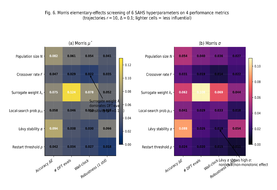
The arrow referring to λ_s sensitivity 0.124 points to the F-row wall-time cell 0.022, and the α high-dispersion arrow points to wall-time 0.019 rather than accuracy σ = 0.088. The embedded annotations cannot support the stated sensitivity interpretations. Original trajectories, response scaling and elementary-effect arrays are required to regenerate and verify the heatmaps.

7.1 The Surrogate Question

The GP-disabled contrast identifies a reported change in the complete search configuration. It does not isolate an additive surrogate-only effect, establish equal accuracy or compare equally engineered surrogate variants for every baseline. Meaningful comparison would charge all parent and gradient calls and record model fitting, candidate screening, cache use and local relaxation separately. This would connect the approximate-model decision to its actual computational consequence.

BH is the closest displayed accuracy comparator, with reported Holm p = 0.18 and mean-rank distance below the corrected CD. This makes it a relevant comparator for a further study, not a proven equivalent or a universally safest method. Parent-model cost can change the practical trade-off, but the present timing record does not quantify that change.

The displayed population-method summaries differ, with GWO having the largest reported final differences. No retained coordinates or event logs isolate its hierarchy as the cause, nor show that every baseline reached an icosahedral structure. The documented LJ₃₈ topology motivates structural diagnostics; it cannot substitute for those diagnostics in the reported runs [29].

PSO’s reported result is conditional on its configuration and task. Cluster-specific revised PSO [9] and crystal-oriented CALYPSO [18] use different structural mechanisms; their existence does not establish a preferred inertia schedule here. A controlled parameter comparison would be needed to attribute the result to the source’s decreasing inertia or other settings.

The Morris record does not justify reducing SAHS tuning to two parameters. A verified screening design could identify priorities within defined ranges, but such priorities would remain conditional on response scaling, task, budget and search randomness. Defaults in Table 1 are reported settings, not deployment recommendations.

7.2 Implications for a Further Comparison

Algorithm selection should connect representation, landscape topology and evaluation work. Candidate studies can compare local-relaxation search, population search and surrogate management under the same admissibility rules and complete resource accounting. For a production electronic model, robust evaluation must include failed SCF calls, gradients and verification of the final geometry. No dimensionality threshold in the retained illustration establishes that CMA-ES is preferable above fifty degrees of freedom, or that any one method is a general default.

A representative test set should contain independently defined systems as well as repeated search seeds, with a prespecified outcome and budget. Thirty searches on one LJ instance and thirty claimed synthetic functions answer different questions. The synthetic archive, task-to-run mapping and full output records are prerequisites to deciding which question the reported statistical comparison actually addresses.

8.1 Internal Validity

Synthetic random-field functions do not reproduce SCF failures, basis effects, chemical symmetries, dissociation boundaries or model–structure errors of real electronic surfaces. Periodic surrogate checks do not remove this mismatch. The source code, complete model archive, energy references, raw outputs and generation logs were not available with the inspected manuscript; the preserved summaries have not been independently regenerated. This evidentiary limitation also applies to the stated calibration and component campaign.

8.2 External Validity

The survey covers representative cluster, conformer, adsorbate and crystal-search literature, while the numerical illustration covers much less. LJ₃₈ has 108 nonrigid degrees of freedom at a nonlinear geometry and is not a low-dimensional example in the usual optimization sense. Its topology alone does not establish dimensionality-dependent rankings or quantitative transfer to other structures. Basis/functional selection is a different model-selection task and is not experimentally addressed here.

8.3 Construct Validity

An energy difference, a basin-success indicator and a structural distance measure different outcomes. A signed difference from an unverified reference cannot be treated as a certified global-optimum gap. A meaningful tolerance criterion requires a matched energy definition and units, while basin classification requires structural information. Reported cost labels must likewise distinguish surrogate calls, true potential calls, electronic SCF cycles and local-minimizer work.

8.4 Statistical Threats

The reported thirty seeds and thirty synthetic functions do not by themselves define independent inferential units or establish power for smaller effects. No documented power calculation supports a fifty-run threshold. BH’s nonrejecting contrast and interval containing zero leave its accuracy difference unresolved rather than proving equivalence. Repeated searches on one structure cannot support a population-wide chemistry claim without a defined sampling model and additional systems.

8.5 Counterarguments and Alternative Readings

SAHS combines established search and surrogate mechanisms, so a claim of algorithmic novelty requires a specified integration rule and comparison to relevant existing hybrids. The component record alone does not provide that proof. Equipping baselines with comparable surrogate management and controlling local-relaxation work would test integration benefits more directly. The canonical LJ₃₈ example remains informative for a landscape discussion, but neither its 108-degree representation nor its known funnels validate a general practical recommendation.

Paired signed-rank inference requires appropriately independent paired differences and, for its usual location interpretation, a suitable symmetry assumption. Shared seed labels are insufficient to establish the pairing or independence of initialized geometries and synthetic functions. Resampling must preserve the actual experimental block, which may be function, seed or a crossed structure. The missing arrays and protocol prevent a certified reanalysis; a future design should define its inferential unit before collecting outputs. Morris variance summarizes variation in elementary effects and can signal nonlinearity or interaction without estimating separate interaction orders [32]. Sobol estimators require a sampling design and sample-size decision; their cost is not generically 2ᵖ or 2¹⁰. For the stated six-parameter, ten-trajectory Morris design the conventional count is seventy calls, and any reduction through reused evaluations needs an explicit log. The retained illustration provides neither that log nor a verified basis for claiming a two-parameter tuning problem.

References

- [1] Podgornik, R. (2007). Energy landscapes: Applications to clusters, biomolecules and glasses (Cambridge molecular science). Journal of statistical physics, 126(2), 423–427. https://doi.org/10.1007/s10955-006-9264-y
- [2] Jensen, F. (2017). Introduction to computational chemistry. John Wiley & Sons. https://www.wiley.com/en-ie/shop/general-chemistry/introduction-to-computational-chemistry-3rd-edition-p-9781118825990
- [3] Henkelman, G., & Jónsson, H. (1999). A dimer method for finding saddle points on high dimensional potential surfaces using only first derivatives. The journal of chemical physics, 111(15), 7010–7022. https://doi.org/10.1063/1.480097
- [4] Storn, R., & Price, K. (1997). Differential evolution – a simple and efficient heuristic for global optimization over continuous spaces. Journal of global optimization, 11(4), 341–359. https://doi.org/10.1023/A:1008202821328
- [5] Eberhart, R., & Kennedy, J. (1995). Particle swarm optimization. Proceedings of the IEEE international conference on neural networks (Vol. 4, pp. 1942–1948). IEEE. https://doi.org/10.1109/ICNN.1995.488968
- [6] Hansen, N., & Ostermeier, A. (2001). Completely derandomized self-adaptation in evolution strategies. Evolutionary computation, 9(2), 159–195. https://doi.org/10.1162/106365601750190398
- [7] Mirjalili, S., Mirjalili, S. M., & Lewis, A. (2014). Grey wolf optimizer. Advances in engineering software, 69, 46–61. https://doi.org/10.1016/j.advengsoft.2013.12.007
- [8] Hartke, B. (1999). Global cluster geometry optimization by a phenotype algorithm with Niches: Location of elusive minima, and low-order scaling with cluster size. Journal of computational chemistry, 20(16), 1752– 1759. https://doi.org/10.1002/(SICI)1096-987X(199912)20:16%3C1752::AID-JCC7%3E3.0.CO;2-0
- [9] Zhou, Y., Zhao, Z., & Cheng, D. (2020). Cluster structure prediction via revised particle-swarm optimization algorithm. Computer physics communications, 247, 106945. https://doi.org/10.1016/j.cpc.2019.106945
- [10] Wales, D. J., & Doye, J. P. K. (1997). Global optimization by basin-hopping and the lowest energy structures of Lennard-Jones clusters containing up to 110 atoms. The journal of physical chemistry a, 101(28), 5111–5116. https://doi.org/10.1021/jp970984n
- [11] Wales, D. J., & Scheraga, H. A. (1999). Global optimization of clusters, crystals, and biomolecules. Science, 285(5432), 1368–1372. https://doi.org/10.1126/science.285.5432.1368
- [12] Goedecker, S. (2004). Minima hopping: An efficient search method for the global minimum of the potential energy surface of complex molecular systems. The journal of chemical physics, 120(21), 9911–9917. https://doi.org/10.1063/1.1724816
- [13] Jin, Y. (2011). Surrogate-assisted evolutionary computation: Recent advances and future challenges. Swarm and evolutionary computation, 1(2), 61–70. https://doi.org/10.1016/j.swevo.2011.05.001
- [14] Liu, X., Yang, Z., Liu, J., Xiong, J., Huang, J., Huang, S., & Fu, X. (2025). Surrogate-assisted global and distributed local collaborative optimization algorithm for expensive constrained optimization problems. Scientific reports, 15(1), 1728. https://doi.org/10.1038/s41598-025-85233-6
- [15] Liu, Y., Liu, J., Jin, Y., Li, F., & Zheng, T. (2023). A surrogate-assisted two-stage differential evolution for expensive constrained optimization. IEEE transactions on emerging topics in computational intelligence, 7(3), 715–730. https://doi.org/10.1109/TETCI.2023.3240221
- [16] Jung, H., Sauerland, L., Stocker, S., Reuter, K., & Margraf, J. T. (2023). Machine-learning driven global optimization of surface adsorbate geometries. NPJ computational materials, 9(1), 114. https://doi.org/10.1038/s41524-023-01065-w
- [17] Yang, Q., Li, Z. Y., Rodríguez-Kessler, P. L., & He, S. G. (2024). Accelerated global optimization of metal cluster structures via the deep neural network complemented with transfer learning and genetic algorithm. Chinese journal of chemical physics, 37(3), 321–329. https://doi.org/10.1063/1674-0068/cjcp2309083
- [18] Wang, Y., Lv, J., Zhu, L., & Ma, Y. (2012). CALYPSO: A method for crystal structure prediction. Computer physics communications, 183(10), 2063–2070. https://doi.org/10.1016/j.cpc.2012.05.008
- [19] Zhu, Z., Yang, Z., Liu, Z., Chen, L., & Cai, X. (2025). State information-driven surrogate-assisted differential evolution for computationally expensive constrained optimization problems. Complex & intelligent systems, 11(8), 359. https://doi.org/10.1007/s40747-025-01980-z
- [20] Rondina, G. G., & Da Silva, J. L. F. (2013). Revised basin-hopping Monte Carlo algorithm for structure optimization of clusters and nanoparticles. Journal of chemical information and modeling, 53(9), 2282–2298. https://doi.org/10.1021/ci400224z
- [21] Carmona, O., Rodríguez-Kessler, P. L., Salazar-Colores, S., & Muñoz-Castro, A. (2025). Revisiting and accelerating the Basin Hopping algorithm for Lennard-Jones clusters: Adaptive and parallel implementation in Python. https://doi.org/10.48550/arXiv.2510.25938
- [22] Behler, J., & Parrinello, M. (2007). Generalized neural-network representation of high-dimensional potential-energy surfaces. Physical review letters, 98(14), 146401. https://doi.org/10.1103/PhysRevLett.98.146401
- [23] Chmiela, S., Tkatchenko, A., Sauceda, H. E., Poltavsky, I., Schütt, K. T., & Müller, K. R. (2017). Machine learning of accurate energy-conserving molecular force fields. Science advances, 3(5), e1603015. https://doi.org/10.1126/sciadv.1603015
- [24] Jinnouchi, R., Karsai, F., & Kresse, G. (2019). On-the-fly machine learning force field generation: Application to melting points. https://doi.org/10.1103/PhysRevB.100.014105
- [25] Pracht, P., Bohle, F., & Grimme, S. (2020). Automated exploration of the low-energy chemical space with fast quantum chemical methods. Physical chemistry chemical physics, 22(14), 7169–7192. https://doi.org/10.1039/c9cp06869d
- [26] Oganov, A. R., & Glass, C. W. (2006). Crystal structure prediction using ab initio evolutionary techniques: Principles and applications. The journal of chemical physics, 124(24), 244704. https://doi.org/10.1063/1.2210932
- [27] Pickard, C. J., & Needs, R. J. (2011). Ab initio random structure searching. Journal of physics: condensed matter, 23(5), 53201. https://doi.org/10.1088/0953-8984/23/5/053201%0A%0A
- [28] Derrac, J., García, S., Molina, D., & Herrera, F. (2011). A practical tutorial on the use of nonparametric statistical tests as a methodology for comparing evolutionary and swarm intelligence algorithms. Swarm and evolutionary computation, 1(1), 3–18. https://doi.org/10.1016/j.swevo.2011.02.002
- [29] Doye, J. P. K., Miller, M. A., & Wales, D. J. (1999). The double-funnel energy landscape of the 38-atom Lennard-Jones cluster. The journal of chemical physics, 110(14), 6896–6906. https://doi.org/10.1063/1.478595
- [30] Macbeth, G., Razumiejczyk, E., & Ledesma, R. D. (2011). Cliff’s delta calculator: A non-parametric effect size program for two groups of observations. Universitas psychologica, 10(2), 545–555. https://doi.org/10.11144/Javeriana.upsy10-2.cdcp
- [31] Hedges, L. V. (1981). Distribution theory for Glass’s estimator of effect size and related estimators. Journal of educational statistics, 6(2), 107–128. https://doi.org/10.3102/10769986006002107
- [32] Morris, M. D. (1991). Factorial sampling plans for preliminary computational experiments. Technometrics, 33(2), 161–174. https://doi.org/10.1080/00401706.1991.10484804
- [33] Virtanen, P., Gommers, R., Oliphant, T. E., Haberland, M., Reddy, T., Cournapeau, D., … Contributors, S. (2020). SciPy 1.0: Fundamental algorithms for scientific computing in Python. Nature methods, 17(3), 261–
- [272] https://doi.org/10.1038/s41592-019-0686-2
- [34] Demšar, J. (2006). Statistical comparisons of classifiers over multiple data sets. The journal of machine learning research, 7, 1–30. https://doi.org/10.5555/1248547.1248548