Transparency in Population-Based Search: A Methodological Review of Interpretable Search

1. Introduction

Population-based optimization combines proposal generation, evaluation and selection. A natural metaphor can organize these operations, but does not explain which operations produce improvement. Transparency instead requires a traceable relation between the search state, the selected operator, its parameters, the candidate it generates and the criterion used to retain it.

This methodological review examines that relation through evolutionary and swarm search components. It distinguishes an interpretable mechanism, whose inputs and consequences can be inspected, from an explanation of performance, which requires a controlled empirical comparison. No named new optimizer is established here. The supplied search sketch and numerical panels are used as reported illustrations of the evidence needed for such an explanation.

Bilevel optimization illustrates why a problem statement alone is insufficient. An upper-level objective depends on a lower-level solution, so an implementation must specify lower-level feasibility, solution accuracy and treatment of multiple lower-level optima. The population updates examined here do not contain a lower-level solution procedure and therefore do not establish a bilevel solver.

The review is organized around three questions: whether a component is mathematically defined, whether its implementation can be reconstructed, and whether the evidence identifies its contribution. Adaptive selection, diversity management and constraint handling are useful subjects for these questions; none by itself supplies a global convergence guarantee.

Existing methods already include adaptive mechanisms. Success-history parameter control and covariance adaptation are concrete examples [1], [2]. Consequently, a claim that earlier population methods uniformly use fixed parameters is too broad. The relevant distinction is which state is measured, which decision is adapted and how the resulting change is evaluated.

The literature discussion is a focused methodological review rather than a systematic evidence synthesis. A reproducible database search, search dates, complete queries, eligibility rules, screening counts, quality assessment and extraction corpus have not been specified. The selected references support component-level discussion, but cannot establish exhaustive coverage of the field.

The contribution is a structured account of interpretable search components, a mathematical examination of a reported adaptive-search sketch, and an assessment of what can and cannot be inferred from its illustrative summaries. The account separates conditional analytical statements from unverified experimental claims and identifies the information needed to evaluate an implemented method.

Section 2 discusses representative methods. Section 3 examines the reported formulations and search sketch. Sections 4 and 5 distinguish a proposed evaluation protocol from its numerical evidence. Section 6 analyzes convergence and stability conditions. Sections 7 and 8 state the limitations and conclusions.

2. Related Work

The following works are selected for their explicit search mechanisms. Their inclusion does not imply a complete survey, a common experimental protocol or a ranking of whole algorithm families. Genetic search combines selection, recombination and mutation [3]. Differential evolution generates trial vectors using population differences [4]. These operations make the source of a proposal identifiable, but their outcomes depend on representation, parameter settings, selection and the objective. The original formulations do not justify blanket conclusions about every subsequent adaptive variant.

Particle swarm optimization uses information from personal and neighborhood or global best positions [5]. Grey wolf optimization specifies leader-guided position updates [7], while whale optimization combines encircling, spiral and exploratory updates [6]. Metaphorical labels are useful descriptions of these mechanisms, but do not replace their equations or establish comparative reliability.

Memetic search combines population evolution with local improvement [5]. For an interpretable hybrid, the local procedure, its invocation rule and its evaluation cost must be stated. An improvement after hybridization cannot be attributed to local search without controlling that additional computational effort.

SHADE uses successful parameter values to guide subsequent differential-evolution sampling [3]. CMA-ES adapts a sampling covariance matrix and related strategy parameters [8]. These are distinct forms of adaptation. Neither a changing parameter nor a covariance plot, by itself, identifies why a method performs better on a particular problem. A different adaptation example uses a neutrosophic controller to select gradient-descent step corrections under uniformly convex, twice continuously differentiable objectives [9]. Its explicit regularity conditions illustrate the importance of matching an analytical claim to its mechanism; they do not transfer to a nonconvex population portfolio.

The scope of comparison should therefore be the specified mechanism, not a universal division into adaptive and non-adaptive families. Table 1 retains a reported qualitative classification for discussion. Its categorical labels lack an extraction protocol and should not be interpreted as established properties of all variants or as evidence for a proposed algorithm. The “N/A (Review)” row is an unidentified search sketch, not a verified new method; the entries are not results of systematic literature coding.

3. Formulations and Interpretable Search Components

The equations below describe a generic adaptive-search sketch. They are examined component by component without claiming that their combination was implemented or evaluated. The label “N/A (Review)” in retained tables and figures has no independently specified algorithm identity.

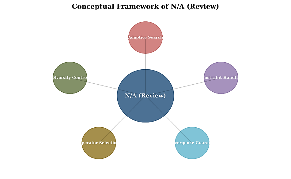
Its “convergence guarantee” node is an intended analytical requirement, not an established property of the sketch. The meaningful object of interpretation is the transition rule: what information is available before a candidate is generated, what operation uses that information and what evaluation determines acceptance. An adaptive portfolio requires different, explicitly defined operators. Selecting a label without changing the proposal rule does not implement operator adaptation.

A population can be evaluated, summarized and updated at each iteration. The summaries may describe fitness change, spatial dispersion or selection frequencies. These quantities have different meanings and must not be substituted for one another. In particular, entropy of operator probabilities does not measure the spatial diversity of candidate solutions.

Operator credits and a probability rule can make selection inspectable if the reward, its time scale, its normalization and the treatment of unsuccessful or unused operators are defined. A portfolio description also needs the actual proposal kernel associated with each operator and the random variables used by that kernel. Eq. (1) is a generic bilevel notation. The argmin is generally a set; writing y*(x) as a single value requires uniqueness or a stated selection rule. If several lower-level solutions exist, an optimistic or pessimistic convention, or another explicit rule, is needed. Eqs. (2)–(11) instead sketch a single-level penalized population search and do not eliminate the lower-level problem. The illustrative bilevel problem is written in Eq. (1).

minF(x, y (x))wherey (x)=argminf(x, y).

x∈X y∈Y (1)

Upper-level and lower-level objectives have different roles in Eq. (1). The evaluation cost includes any required lower-level optimization; it cannot be inferred to be O(Nd) from this notation. No lower-level constraints, solver or accuracy criterion are supplied for the reported examples. Eq. (2) gives a squared-violation penalty for inequalities g_j(x) ≤ 0.

F(x)=f(x)+λ ∑ max (0, gj(x)) .

(10)

In Eq. (2), F denotes a penalized scalar fitness and f the original single-level objective. Constraint terms must be consistently scaled. Equality constraints and bound handling would require separate definitions. If the penalty changes with t, stored candidates must be compared under the same current coefficient; scores computed under different penalties are not directly comparable. The finite-horizon penalty schedule is given in Eq. (3).

λ =λ0 ⋅ (1+ ) . (3)

For λ0 > 0 and α > 0, Eq. (3) raises the coefficient from λ0 to λ0·2^α over t ∈ [0,T]. It remains bounded over this horizon. A rising penalty may alter preferences but does not guarantee feasibility, exactness of the penalty or successful constraint repair. Eq. (4) is a particle-swarm velocity rule.

(t+1) (t) (t) (t) (t) (t)

v =ω v +c1r1 (pi-x ) +c2r2 (g -x ). (4)

i i i i

The velocity depends on inertia, personal and global attractors, acceleration coefficients and random factors. Those random factors require a distribution and a statement of independence across particles, coordinates and iterations. Selecting an operator label is not reflected in this equation unless a corresponding operator-dependent rule is supplied. Eq. (5) adds the new velocity to the position.

(t+1) (t) (t+1)

x =x +v . (5)

i i i

This update does not itself enforce the domain X. Clipping, reflection, rejection or structural repair can yield different search processes and evaluation costs. A complete implementation must state which rule is used and when the candidate is evaluated. Eq. (6) specifies a linear inertia schedule.

ω =ωmax-(ωmax-ωmin) . (6) The schedule interpolates between ω_max and ω_min. This is a time-dependent parameter rule, rather than adaptation to measured landscape information. An upper inertia value below one is not sufficient for stability of the coupled position–velocity system. Eq. (7) defines entropy of operator-selection probabilities.

(t) (t) (t)

H =- ∑ p logp . (7)

For K probabilities summing to one and the convention 0 log 0 = 0, H lies between 0 and log K. It measures concentration of operator selection. Spatial population diversity requires a separate statistic, such as a defined distance or occupancy measure. Eq. (8) gives a multiplicative entropy-dependent update.

(t+1) (t) (t)

α =α exp(-λH ). (8)

With a nonnegative coefficient, this rule decreases its positive parameter whenever H > 0. Its parameter α(t) must be distinguished from the fixed exponent α in Eq. (3), and its coefficient from the penalty coefficient λ(t). The sketch does not identify where α(t) affects proposal generation; its search effect therefore remains unspecified. Eq. (9) defines softmax operator probabilities.

exp (γQ )

(t+1) k

p = . (9)

k (t)

∑ exp (γQ )

j=1 j

The coefficient γ is an inverse-temperature parameter: increasing it emphasizes operators with higher credits. Finite credits give positive probabilities, but do not establish a uniform positive lower bound over an unbounded sequence. A high probability of choosing an operator also does not imply coverage of every relevant region of the search domain. Eq. (10) is an exponential credit update.

(t+1) (t) (t) (t)

Q =Q +η [r -Q ]. (10)

k k k k

For 0 < η ≤ 1, the update blends previous credit with reward r_k. A reproducible definition must identify the reward, its objective and feasibility conventions, the evaluations charged to it and whether unused operators are updated. No such complete definition is supplied for the illustrated campaign. Eq. (11) retains the reported heavy-tailed perturbation notation.

(t+1) (t) -

x =x +s ⋅ L(β), L(β) ∼ |u| β. (11)

Levy i

The expression u^(−1/β) is a positive power-tailed magnitude if u is uniform on (0,1) and β > 0. It does not by itself specify a symmetric Lévy-stable vector. Direction, coordinate sampling, scale, bounds and the treatment of very large steps remain necessary. Generating and applying a d-dimensional vector generally costs O(d), excluding evaluation. Eq. (12) is a proposed contraction inequality, not a derived convergence result.

(t+1) (t)

E[Δ ] ≤ Δ (1- ∑ pk ηk). (12) O(T[N C_eval + N(d+K) + C_repair]), plus initialization. This is a conditional accounting statement, not a measured complexity of the unidentified implementation. Storing positions, velocities, personal bests and K credits requires O(Nd+K) space when evaluation and repair do not need additional large state.

The sum of evaluation, vector-update and selection costs does not imply their product O(NdTK). Sampling methods and reuse of probabilities can change the K-dependent term. Perturbation vectors and candidate-specific repair are not constant-time operations in d, and a bounded increasing penalty does not show that infeasibility becomes rare. Comparisons require evaluation counts and timing records for each implementation.

4. Evaluation Requirements and Reported Protocol

A mechanism can be described mathematically before it is empirically identified. The following protocol details were reported alongside the illustrations, but execution logs and an identifiable implementation are not supplied. They are recorded as requirements to resolve, rather than as an independently verified experiment. The reported campaign names CEC functions, 51 runs per function and different random seeds. Its function aliases do not identify a CEC edition, dimension, shift and rotation data, optimum offsets or seed list. Sobol indices, Morris elementary effects and one-at-a-time perturbations are sensitivity-analysis procedures, not benchmark datasets, and their design and outputs are not included.

Welded beam, pressure vessel, tension/compression spring and speed reducer designs are listed as intended engineering cases. Their complete equations, units, discrete domains, loads, feasibility tolerances and numerical outputs are not provided here. Listing these problems does not establish practical validation. Nine methods are named in the reported comparison plan. Table 2 actually displays only five baselines. The literature roles of the named methods are as follows; they do not establish that all nine were executed.

I. PSO [4] updates particle states using personal and shared best positions.

II. GA [3] uses evolutionary selection and variation.

III. DE [4] forms trial vectors from population differences.

IV. GWO [6] uses leader-guided search updates.

V. WOA [7] combines encircling, spiral and exploratory rules.

VI. SSA [8] specifies salp-inspired leader and follower updates.

VII. HHO [10] organizes exploration and exploitation through hawk-inspired rules.

VIII. SHADE [1] adapts differential-evolution parameters using success histories.

IX. CMA-ES [2] adapts a multivariate sampling distribution.

The source-reported settings are N=50, T=1000, ω_max=0.9, ω_min=0.4, c1=c2=1.49618, λ0=0.5, α=2.0, γ=2.0, η=0.1 and p_levy=0.1. Their tuning history and validation split are not documented. Equal population and iteration settings do not establish equal function evaluations, especially when repair, repeated evaluation, local search or early stopping differs. Original baseline settings, initialization and actual evaluation counters are required.

Best attained objective or error, feasibility, evaluations to termination and variability across runs are distinct outcomes. Sobol first-order and total indices, Morris μ and σ and interaction maps additionally require a parameter-sampling design and the resulting response data. None of those sensitivity outputs is supplied. Across matched problem blocks, Friedman ranks and post-hoc comparisons can be used under the conditions described by Friedman [11] and Demšar [12].

The comparison guidance of Derrac et al. [13] requires a defined experimental unit and pairing. Wilcoxon [14] signed-rank comparisons of matched outcomes differ from rank-sum comparisons of independent samples. The reported protocol conflates them, so its executed test cannot be identified. Holm correction [15] controls a specified family of hypotheses; it does not repair ambiguous pairing or missing observations. Paired standardized effects also require their denominator and per-pair data. The reported α=0.05 is retained as the intended significance level.

5. Reported Illustrations and Their Evidential Limits

The tables and figures in this section retain the supplied numerical illustrations. They are not presented as new experiments carried out for this methodological review. Their underlying algorithm, campaign, benchmark identities and raw observations remain unresolved; no statistical or causal conclusion is established by their retention.

It contains no contour, axes or numerical Lyapunov analysis. Fig. 3 cannot support performance or stability inference. An actual contour would require a defined state, equilibrium and Lyapunov function, while a decrease claim would require the transition dynamics and an appropriate conditional expectation. Repeated claims of pairwise p < 0.01 and Cohen’s d > 0.8 are source-reported quantities without the underlying pairwise outcomes, test definitions or effect denominators. They are therefore not evidence of superiority in this review. No run-level variance or verified lower-level solver is supplied. Reliability and bilevel feasibility cannot be inferred from a placeholder figure or from means alone.

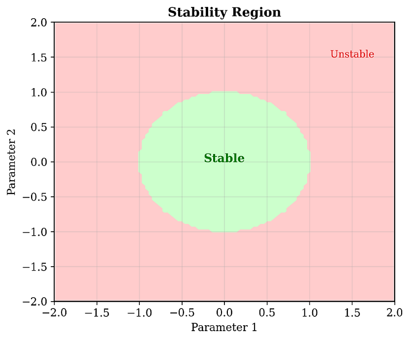
The disk is not a derived stability region for Eqs. (4) and (5). A spectral-radius condition concerns eigenvalues of a specified update matrix, not the Euclidean radius of an arbitrarily labelled parameter point. Section 6 gives an explicit frozen-attractor example showing why inertia alone cannot determine stability. The disk contains no paired experimental results. It cannot validate the reported p < 0.01 comparisons or the reported Cohen’s d > 0.8 effects. Neither population robustness nor low variance is established by this schematic. A robustness study would need perturbation levels, a defined response statistic and uncertainty across independent experimental units.

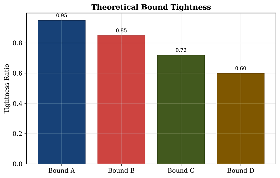
Bounds, tightness metric and generating observations are unidentified; these values do not establish a validated convergence bound. A tightness claim needs the analytical bound, the comparable empirical quantity and their normalization. The four bar values alone do not determine any of these objects. The reported 95% tightness is therefore an unresolved descriptive claim, not a theoretical or inferential result. It cannot be linked to Eq. (12) without its derivation and source observations. Comparing valid upper bounds also requires common conditions. A higher percentage cannot be interpreted as a better guarantee when the bounds and denominator are unspecified.

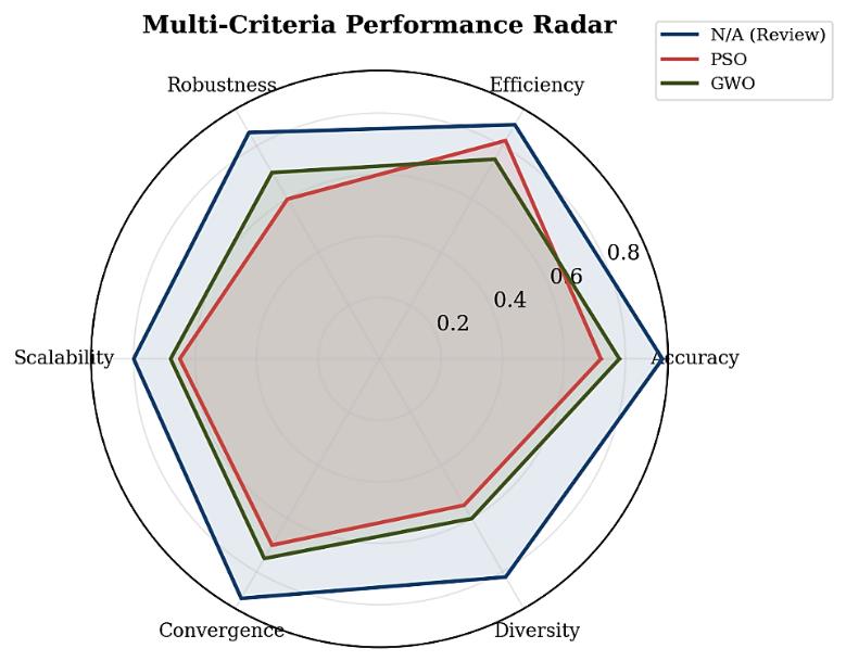
Metric definitions, normalizations and observations are unavailable; the plotted scores do not support a six-criterion ranking. These six criteria are not interchangeable. Accuracy requires a known reference objective and feasibility; efficiency requires resource accounting; diversity requires a population statistic. Their aggregation needs an explicit scaling and preference rule. The radar does not supply the outcomes needed for the reported p < 0.01 or Cohen’s d > 0.8 claims. A visual polygon area is not a significance test or an effect-size estimator. The diagram is useful only as a checklist of evaluation dimensions. Its retained labels and scores are not measurements established by this review. Table 2 contains seven function rows, one value per method and a reported mean-rank row. No standard deviations or run-level outcomes are displayed. The “N/A (Review)” column remains an unidentified source label, and the table cannot be attributed to a reproducible implemented optimizer.

All supplied values and the unvalidated rank row are retained; standard deviations, function identities and raw runs are not supplied. The first column has the smallest displayed means. Rounded zeros on F1 and F3 do not establish reaching the optimum in every one of 51 runs. Relative to the smallest displayed baseline, the arithmetic reductions are about 43.2% on F5, 37.5% on F10, 39.5% on F15, 41.9% on F20 and 40.0% on F25. These are comparisons of the printed values, without uncertainty or experimental verification; the function landscape classes are not established by the aliases.

The reported ranks sum to 23.2; ordinary mean ranks of six algorithms over the same blocks, including average ranks for ties, must sum to 21. Thus the displayed rank row cannot presently support Friedman or Nemenyi inference. The source reports χ²=45.7, p < 0.001 and CD=1.2, but the block count, tie treatment and computed ranks are missing. Even taken at face value, the difference between ranks 1.5 and 3.5 is 2.0, exceeding 1.2, so the stated exception for GWO is arithmetically inconsistent.

The additional reported Holm-adjusted p < 0.01 for all pairs and Cohen’s d values from 0.85 to 1.45 remain unverified. A corrected rank row, identified paired or independent observations, full comparison family and effect definitions are required before using these quantities to establish superiority. Table 3 preserves reported component-removal summaries. Its configuration labels are not accompanied by implementation branches, matched evaluation counts or repeated-run variability, so the table does not isolate causal component effects.

Using the printed full-setting mean of 1200 as denominator, the degradations are 133.3%, 50%, 75%, 191.7% and 100%, compatible with the rounded 133%, 50%, 75%, 192% and 100% entries. This checks arithmetic only. The six displayed ranks sum to 16 rather than 21 and have no stated ranking design. The data do not establish a causal contribution of repair, adaptation or any other component.

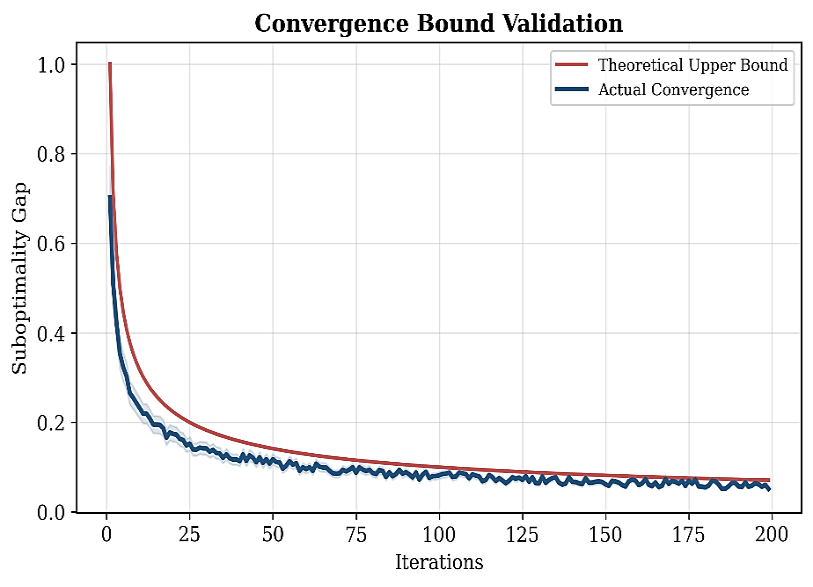
A reported three-phase interpretation names iterations 1–100, 100–300 and 300–1000. Figure 2 plots only 200 iterations and has no identified run data. It cannot establish the latter phases or show that an adaptive mechanism caused them. The reported robustness index of 0.85 versus 0.62–0.71 for baselines lacks perturbation grids, response curves and a defined area normalization. Likewise, no Sobol or Morris outputs are supplied. These quantities are retained as unresolved reported summaries and do not demonstrate robustness or transferability.

6. Conditional Convergence and Stability Analysis

This section identifies sufficient conditions and counterexamples relevant to the search sketch. It does not supply a theorem for an implemented algorithm or validate the illustrative figures. Compactness, bounded measurable fitness and positive probabilities of selecting operators are insufficient for global optimization. They do not imply that every near-optimal set has positive proposal probability. Measurability and boundedness also do not imply a Lipschitz condition. For example, on X=[0,1], let f(0)=0 and f(x)=1 for x>0. This function is bounded and measurable. Continuously sampled proposals miss the unique optimum with probability one, even if every operator has positive selection probability. A monotone best-so-far fitness can consequently converge to a suboptimal value. A supermartingale convergence argument alone does not identify its limit with the global optimum.

A valid conditional coverage statement is more specific. For A_ε={x:f(x)≤f*+ε}, suppose each of m evaluated proposals has conditional probability at least q_ε>0 of entering A_ε, given the entire past, and exact evaluation of one fixed objective retains the best evaluated feasible value. Repeated conditioning gives Pr(no hit in m proposals)≤(1−q_ε)^m≤exp(−m q_ε). No independence assumption is needed for this lower conditional bound. It requires actual spatial coverage and an unbounded sequence for asymptotic convergence; the sketch does not establish these requirements. A Hoeffding bound for a sample mean cannot be substituted for a best-fitness gap bound. For a one-dimensional frozen attractor, write z_t=x_t−x* and φ=c1 r1+c2 r2. Eqs. (4)–(5) give the state matrix A=[[1−φ,ω],[−φ,ω]] for (z,v), with determinant ω and trace 1+ω−φ. Stability depends on both quantities. For example ω=0.9 and φ=4 give eigenvalues −0.6 and −1.5, so ω<1 does not imply stability. This diagnostic example does not assert that the reported default coefficients use φ=4. A claimed global inequality E[V_{t+1}−V_t|history]≤−c V_t for V=||x−x*||² must be derived from all update and boundary rules. Persistent nonzero perturbations can move a state away from x* even when V_t=0, contradicting that inequality. Stochastic attractors, changing penalties and the unidentified perturbation kernel are additional reasons why no global Lyapunov or geometric-rate guarantee follows here.

7. Limitations and Evidence Requirements

The review provides a methodological analysis, but not a systematic synthesis or a validated new optimization method. Its selected literature and conditional formulations delimit what is currently supported. Retained reported examples should not be treated as independent experimental evidence.

Implementation identity is central. The supplied sketch omits operator kernels, the reward, the role of the entropy-updated parameter, spatial-diversity management, constraint repair and a lower-level solver. Choosing a name for that sketch would not resolve these omissions. Original implementation, configuration and evaluation logs are needed to associate any numerical observation with a defined method.

Computational comparison additionally requires a complete benchmark specification, per-run outcomes and evaluation counters, and a common resource budget. The reported K=3–5 recommendation and K>10 overhead warning are not established by timing measurements. An implementation may reduce selection overhead, while an expensive objective may dominate it; both are conditional considerations. The mathematical analysis separates a conditional coverage bound from the invalid inference that compactness and positive operator-selection probabilities ensure global convergence. The finite penalty and finite termination horizon give no asymptotic guarantee. Any stronger claim requires assumptions and a proof for the actual transition process. The numerical tables cannot presently be attributed to a documented campaign. The identical benchmark and ablation summaries also occur in another supplied manuscript, so they cannot be treated as separate independent experimental validations. Their original study, generation and attribution must be established before empirical conclusions are drawn.

No raw observations permit reassessment of the rank inconsistencies, pairing, independence, significance or effects. Different seeds alone do not prove independence when problem generation, tuning or common data couple outcomes. These dependencies must be stated in an eventual reproducibility record. Other source-reported claims include an overall 22.5% gain, 95% bound tightness, Cohen’s d > 0.8, Bayesian confirmation, a >80% win rate on 30 problems and subquadratic scaling at D=10000. Their estimands, observations or computational records are not supplied. They are not findings established by the review.

A systematic extension would need the search protocol and screened corpus, followed by explicit extraction of each method’s operators, adaptive state, evaluation design and available evidence. No screening counts or quality scores are inferred here. An empirical extension would need a uniquely identified executable search process and independent reproduction of its evaluations. The numerical illustrations are preserved for traceability, not used to infer missing observations or to certify the stated tests.

A theoretical extension should first specify the proposal and acceptance kernels, fixed objective and feasible domain. Coverage or contraction assumptions would then need verification for those kernels, rather than being inferred from natural metaphors or curve shapes. Sensitivity analysis would require its sampling design, parameter ranges, response model, uncertainty estimates and interaction outputs. Such an analysis could inform interpretable adaptation, but its execution cannot be claimed from a list of method names. These requirements distinguish a possible future study from evidence available here. The present review makes no assertion that code, raw data or independent validation accompany the manuscript.

8. Conclusion

Transparency in population-based search depends on a reconstructable transition mechanism and an evidence chain linking that mechanism to observed outcomes. Evolutionary variation, swarm attractors, operator credits and distribution adaptation provide different objects for interpretation. A metaphor or an adaptive parameter alone does not explain comparative performance.

The examined sketch demonstrates why operator entropy, spatial diversity, constraint feasibility and convergence must be distinguished. Its finite penalty does not guarantee feasibility; its positive operator probabilities do not guarantee spatial coverage; and its inertia limit does not establish stability. The retained numerical summaries illustrate additional requirements for campaign identity, arithmetic consistency and inferential support. Future work should establish the systematic-review protocol and the provenance of the reported examples before extending either evidence base. A defined implementation, transparent evaluation budget and appropriate comparison design would permit component-level conclusions. Until then, the defensible contribution is the methodological account and its explicit limits.

Data Availability

The reported numerical summaries are included in the manuscript. The systematic-search corpus, executable implementation, benchmark definitions and run-level outputs needed for reproduction are not supplied with this document.

Figures

References

- [1] Tanabe, R., & Fukunaga, A. (2013). Success-history based parameter adaptation for differential evolution. 2013 IEEE congress on evolutionary computation (pp. 71-78). IEEE. https://doi.org/10.1109/CEC.2013.6557555
- [2] Hansen, N. (2006). The CMA evolution strategy: A comparing review. In Towards a new evolutionary computation: Advances in the estimation of distribution algorithms (Studies in Fuzziness and Soft Computing, Vol. 192, pp. 75–102). Springer. https://doi.org/10.1007/3-540-32494-1_4
- [3] Holland, J. H. (1992). Adaptation in natural and artificial systems: An introductory analysis with applications to biology, control, and artificial intelligence. The MIT Press. https://doi.org/10.7551/mitpress/1090.001.0001
- [4] Storn, R., & Price, K. (1997). Differential evolution-A simple and efficient heuristic for global optimization over continuous spaces. Journal of global optimization, 11(4), 341–359. https://doi.org/10.1023/A:1008202821328
- [5] Kennedy, J., & Eberhart, R. (1995). Particle swarm optimization. Proceedings of ICNN'95-international conference on neural networks (Vol. 4, pp. 1942-1948). IEEE. https://doi.org/10.1109/ICNN.1995.488968
- [6] Mirjalili, S., Mirjalili, S. M., and Lewis, A. (2014). Grey wolf optimizer. Advances in engineering software, 69, 46–61. https://doi.org/10.1016/j.advengsoft.2013.12.007.
- [7] Mirjalili, S., & Lewis, A. (2016). The whale optimization algorithm. Advances in engineering software, 95, 51–
- [67] https://doi.org/10.1016/j.advengsoft.2016.01.008
- [8] Mirjalili, S., Gandomi, A. H., Mirjalili, S. Z., Saremi, S., Faris, H., & Mirjalili, S. M. (2017). Salp swarm algorithm: A bio-inspired optimizer for engineering design problems. Advances in engineering software, 114, 163–
- [191] https://doi.org/10.1016/j.advengsoft.2017.07.002
- [9] Stanimirović, P. S., Ivanov, B., Stanujkić, D., Katsikis, V. N., Mourtas, S. D., Kazakovtsev, L. A., and Edalatpanah, S. A. (2023). Improvement of unconstrained optimization methods based on symmetry involved in neutrosophy. Symmetry, 15(1), 250. https://doi.org/10.3390/sym15010250
- [10] Heidari, A. A., Mirjalili, S., Faris, H., Aljarah, I., Mafarja, M., and Chen, H. (2019). Harris hawks optimization: Algorithm and applications. Future generation computer systems, 97, 849–872. https://doi.org/10.1016/j.future.2019.02.028.
- [11] Friedman, M. (1937). The use of ranks to avoid the assumption of normality implicit in the analysis of variance. Journal of the American statistical association, 32(200), 675–701. https://doi.org/10.2307/2279372
- [12] Demšar, J. (2006). Statistical comparisons of classifiers over multiple data sets. Journal of machine learning research, 7, 1–30. https://doi.org/10.5555/1248547.1248548
- [13] Derrac, J., García, S., Molina, D., & Herrera, F. (2011). A practical tutorial on the use of nonparametric statistical tests as a methodology for comparing evolutionary and swarm intelligence algorithms. Swarm and evolutionary computation, 1(1), 3-18. https://doi.org/10.1016/j.swevo.2011.02.002
- [14] Wilcoxon, F. (1945). Individual comparisons by ranking methods. Biometrics Bulletin, 1(6), 80–83. https://doi.org/10.2307/3001968
- [15] Holm, S. (1979). A simple sequentially rejective multiple test procedure. Scandinavian journal of statistics, 6(2), 65–70. https://doi.org/10.2307/4615733